1817
Simulation Evidence for use of a Denoising Auto-Encoder (DAE) to Improve Ultra-Low Field (64mT) MRI with a High Field (3T) Prior1Biomedical Engineering, Electrical & Software Engineering, Radiology, University of Calgary, Calgary, AB, Canada, 2Hotchkiss Brain Institute, Foothills Medical Centre, Calgary, AB, Canada
Synopsis
In this work, the denoising autoencoder is applied to simulated low field, low resolution, low signal-to-noise images and used to recover the high field, high resolution, high signal-to-noise paired image. Different types of noise, gaussian and chi-squared, is added in simulation. We found that the denoising autoencoder worked slightly better for normally disturbed noise, but not in all cases. We found a linear trend between the model performance with RMSE and the standard deviation of the added noise. This work demonstrates the use of simple and robust denoising autoencoder to improve low field MRI.
Introduction
Low field MRI scanners are >20x less expensive than 3T MRI scanners over a ten-year period; they have a dramatically smaller footprint (>15x); have much lower energy consumption (~60x less electricity) [1]; have notably lower fields than 1.5T or 3T (e.g., 65mT), which reduces energy absorption in the subject; and they do not require liquid helium [2].Low-field MRI can produce images, but they are starved with low signal-to-noise-ratio (SNR) [3]. Machine learning is particularly useful in denoising images when a paired high-SNR image is available for training [4,5]. In this work we will apply a denoising autoencoder (DAE) [6] to reduce the noise in simulated low-field MRI.
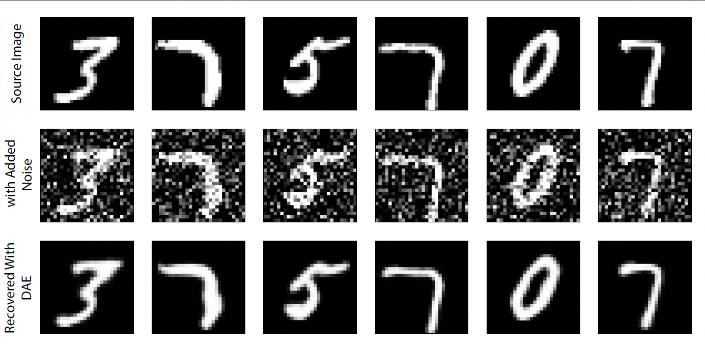
The classical implementation of the DAE uses the MINST (Modified National Institute of Standards and Technology) hand written number dataset [7,8], a series of numbers in 28x28 grid of greyscale images. In such an experiment, low noise images are available, which are used as the targets and random noise is added to them, and these images are used as the input to the model. The model is then trained to remove the noise from the input images and return a lower noise output. Figure 1 demonstrates a DAE applied to the MNIST dataset.
We hypothesize that the denoising autoencoder will be a useful, simple-to-use denoising algorithm, that can be applied to the image domain MRI to generate low-noise images from high noise cases. We show this with a simple and replicable implementation. We explore the problem with different noise types and levels. In effect we aim to use this machine learning implementation to estimate high SNR, high resolution, high field, MRI from low SNR, low resolution, low field MRI.
Methods
In this study we use the IXI database [9]. We use only a portion of the images from the higher field 3T, and these were curated to just 70 participants. These images have a resolution of 1mmx1mmx1mm.We reduce the resolution of these images to those expected from low field MRI, to have resolutions of 1.5mmx1.5mmx5mm. Then we add noise based on the 7/4 power law relationship [10]. At low field the SNR can become dominated by electronics, so we add noise at several levels. We add this noise in two forms, one with normally distributed noise, and one with Chi-squared distribution [11,12] (a more generalized version of Rician noise [13]), with the later more accurately depicting noise found in MRI. In general, most previous DAE experiments only explore normally distributed noise. We add noise in three levels, with standard deviations of 250, 500 and 750.
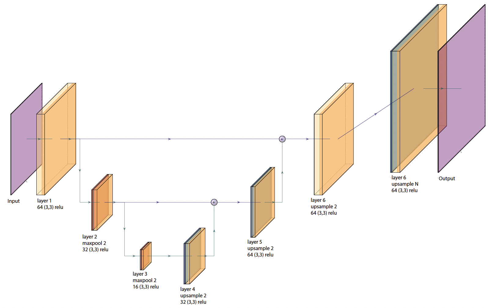
To build the autoencoder model, we define a simple convolutional neural network (CNN) architecture, shown in Figure 2. This architecture has 7 total layers in a U-net style configuration, with the latent space becoming smaller towards the bottom of the U. We also use skip connections, as we found this reduced blurring of the DAE output. We split the data by participant, with 80% of the data used in training and 20% used in validation. The root mean square error (RMSE) images are used as the performance metric.
Results
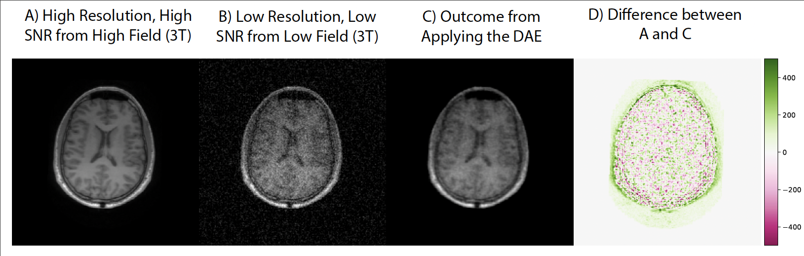
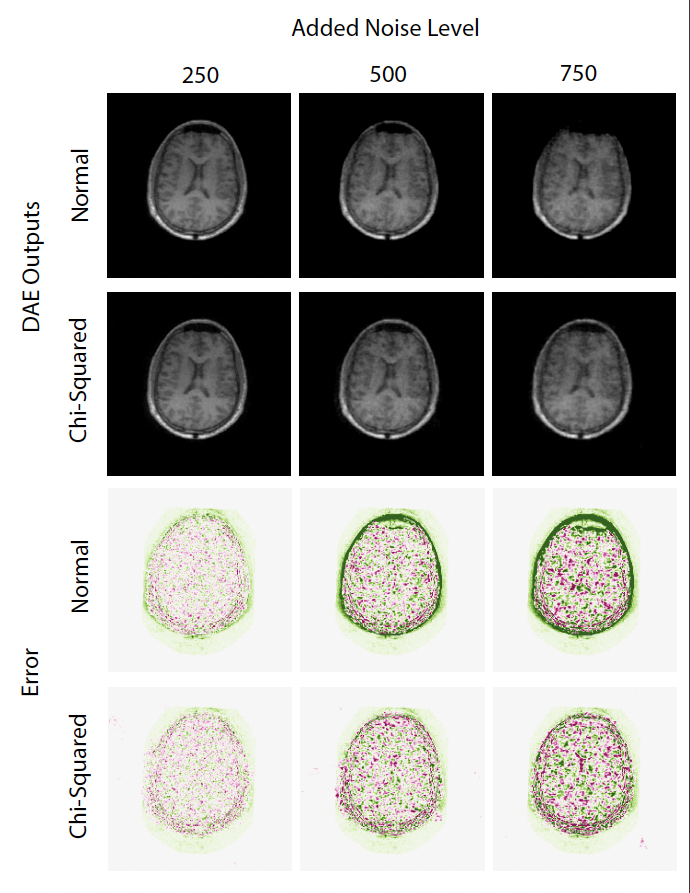
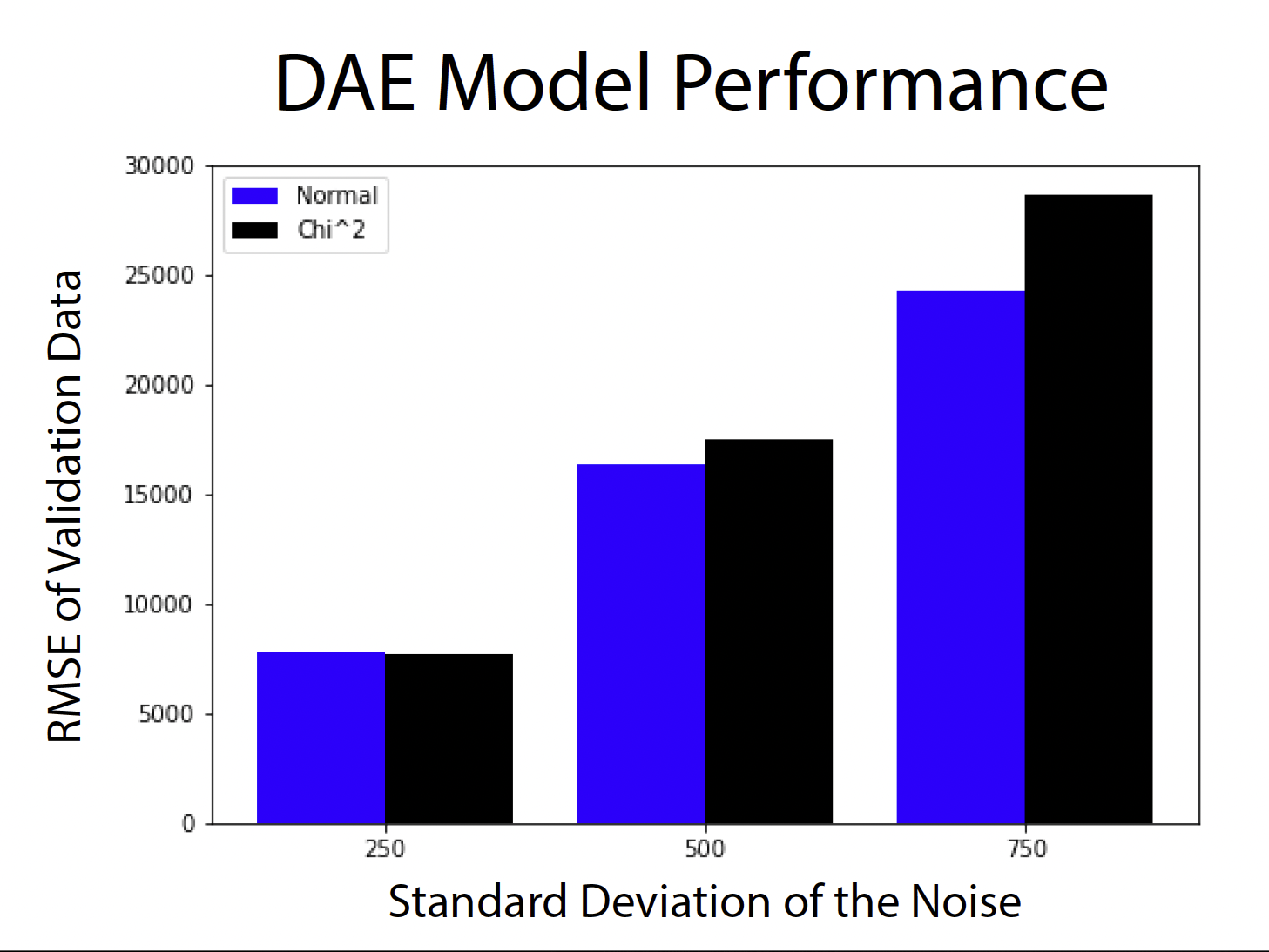
Figure 3 shows representative images of the high-field, high resolution 3T images, simulated low field, low resolution 64mT images, and the output of the auto encoder and difference to the target images. Figure 4 shows a panel of the performance for different noise levels and types. Here we see the image quality deteriorating and the error growing with the amount of added noise as we would expect. Figure 5 shows performance on all the validation data, we observe here that the DAE performs marginally better with normally distributed noise than with a chi-squared distribution. A linear relationship is observed between the standard deviation and the performance of the DAE.Discussion
This work shows how the denoising autoencoder can reduce the noise and improve the quality of the images, however, this requires a high-SNR prior. Most DAE implementations in realms outside of medical imaging using a Gaussian or normally distributed additive noise, here we look at the impact of using a Chi-squared distributed noise to better understand the problem from the perspective of the MRI scientist --- Although there was some, loss in performance with Chi-squared noise, the model still performed well.A limitation of this simulation is that it does not consider motion that might exist between the image pairs, which could be simulated in future work. Further, future work should also include the gathering of empirical data, for example – low field and high field images pairs to minimise errors that might exist due to a simulation. Careful execution of the head placement during the collection of the pairs so that alignment is similar should be considered. However, this work helps to motivate that more costly experiment. Another limitation in this simulation is that we do not consider T1&T2 differences at different field strengths.
Conclusion
It can be concluded that the denoising auto-encoder is a simple and effective way to denoise images from low field MRI and obtain images closer to those acquired at 3T. Gaussian noise performs marginally better with the autoencoder, but Chi-squared noise can also be removed satisfactorily.Acknowledgements
No acknowledgement found.References
1. Heye, T., et al., The energy consumption of radiology: energy-and cost-saving opportunities for CT and MRI operation. Radiology, 2020. 295(3): p. 593-605.
2. Marques, J.P., F.F. Simonis, and A.G. Webb, Low‐field MRI: An MR physics perspective. Journal of magnetic resonance imaging, 2019. 49(6): p. 1528-1542.
3. Wald, L.L., et al., Low‐cost and portable MRI. Journal of Magnetic Resonance Imaging, 2020. 52(3): p. 686-696.
4. Antun, V., et al., On instabilities of deep learning in image reconstruction and the potential costs of AI.Proceedings of the National Academy of Sciences, 2020. 117(48): p. 30088-30095.
5. Coupé, P., et al., Robust Rician noise estimation for MR images. Medical image analysis, 2010. 14(4): p. 483-493.
6. Pinaya, W.H.L., et al., Autoencoders, in Machine learning. 2020, Elsevier. p. 193-208.
7. KERAS. Convolutional autoencoder for image denoising. 2021; Available from: https://keras.io/examples/vision/autoencoder/.
8. LeCun, Y., et al., Gradient-based learning applied to document recognition. Proceedings of the IEEE, 1998. 86(11): p. 2278-2324.
9. IXI. Information eXtraction of Images Database Website. 2017; Available from: http://brain-development.org/ixi-dataset/.
10. Haacke, E.M., et al., Magnetic Resonance Imaging: Physical Principles and Sequence Design. 1999: Wiley-Liss.
11. Kay, S.M., Fundamentals of Statistical Signal Processing: Detection Theory. 1998: Prentice Hall Signal Processing Series.
12. Kay, S.M., Fundamentals of Statistical Signal Processing: Estimation Theory. 1993: Prentice Hall Signal Processing Series.
13. Gudbjartsson, H. and S. Patz, The Rician distribution of noisy MRI data. Magnetic resonance in medicine, 1995. 34(6): p. 910-914.
Figures