1763
Deep subspace transfer learning for SMS image reconstruction from single-slice training: Application to CMR Multitasking1Biomedical Imaging Research Institute, Cedars-Sinai Medical Center, Los Angeles, CA, United States, 2Department of Bioengineering, University of California, Los Angeles, Los Angeles, CA, United States
Synopsis
CMR multitasking is promising for quantitative cardiac imaging, and can achieve fast three-slice quantification when combined with simultaneous multi-slice (SMS) acquisition. However, slow non-Cartesian iterative reconstruction is a barrier to clinical adoption. Deep learning can accelerate reconstruction, but the SMS training data are currently limited. Here we propose a data-consistent deep subspace transfer learning strategy that trains on single-slice T1 CMR multitasking data but is applied to SMS-encoded T1 CMR multitasking image reconstruction. The proposed strategy is >40x faster than the conventional SMS reconstruction, resulting in an equally better image quality and comparably precise T1 as in single-slice reconstruction.
Introduction
CMR multitasking is a promising approach for quantitative imaging without ECG or breath-holds1. In combination with simultaneous-multi-slice (SMS) acquisition, CMR multitasking offers fast three-slice quantification in a fraction of the time of standard methods2,3. However, slow iterative non-Cartesian reconstruction is still a barrier to clinical adoption. Single-slice CMR multitasking has reached clinically applicable reconstruction times through deep subspace learning reconstruction4, but this required hundreds of training scans; equally large SMS data are not yet available. We propose a data-consistent (DC) deep subspace transfer learning strategy that trains on pre-existing single-slice data but is applied to SMS-encoded data. The proposed method can accelerate SMS T1 multitasking reconstruction by >40x without any SMS training data.Theory
CMR multitasking reconstructionIn CMR multitasking, a dynamic image is represented as a low-rank tensor $$$\mathcal{X}$$$ decomposed into a spatial factor matrix $$$\mathbf{U}$$$ and a low-rank temporal factor tensor $$$\it{\Phi}$$$ according to $$$\mathcal{X}=\it{\Phi}\times_\mathrm{1}\mathbf{U}$$$.1 The most time-consuming step is solving $$$\mathbf{U}$$$:$$\widehat{\mathbf{U}}=\arg\min_{\mathbf{U}}\left\|\mathbf{b}-\mathit\Omega\left(\mathit\Phi\times_{1}\mathbf{F}_{\mathrm{NU}}\mathbf{S U}\right)\right\|_{2}^{2}+\lambda R(\mathbf{U})\tag{1}$$
Here $$$\mathbf{b}$$$ is the acquired data, $$$\mathbf{F}_{\mathrm{NU}}$$$ is the non-uniform Fourier transform, $$$\mathbf{S}$$$ applies sensitivity maps, $$$\mathit\Omega$$$ is the k-t space undersampling operator, and $$$R$$$ is a regularization functional such as a wavelet sparsity penalty. Conventionally, Eq. (1) is solved by slow iterative methods.
Non-Cartesian DC deep subspace learning
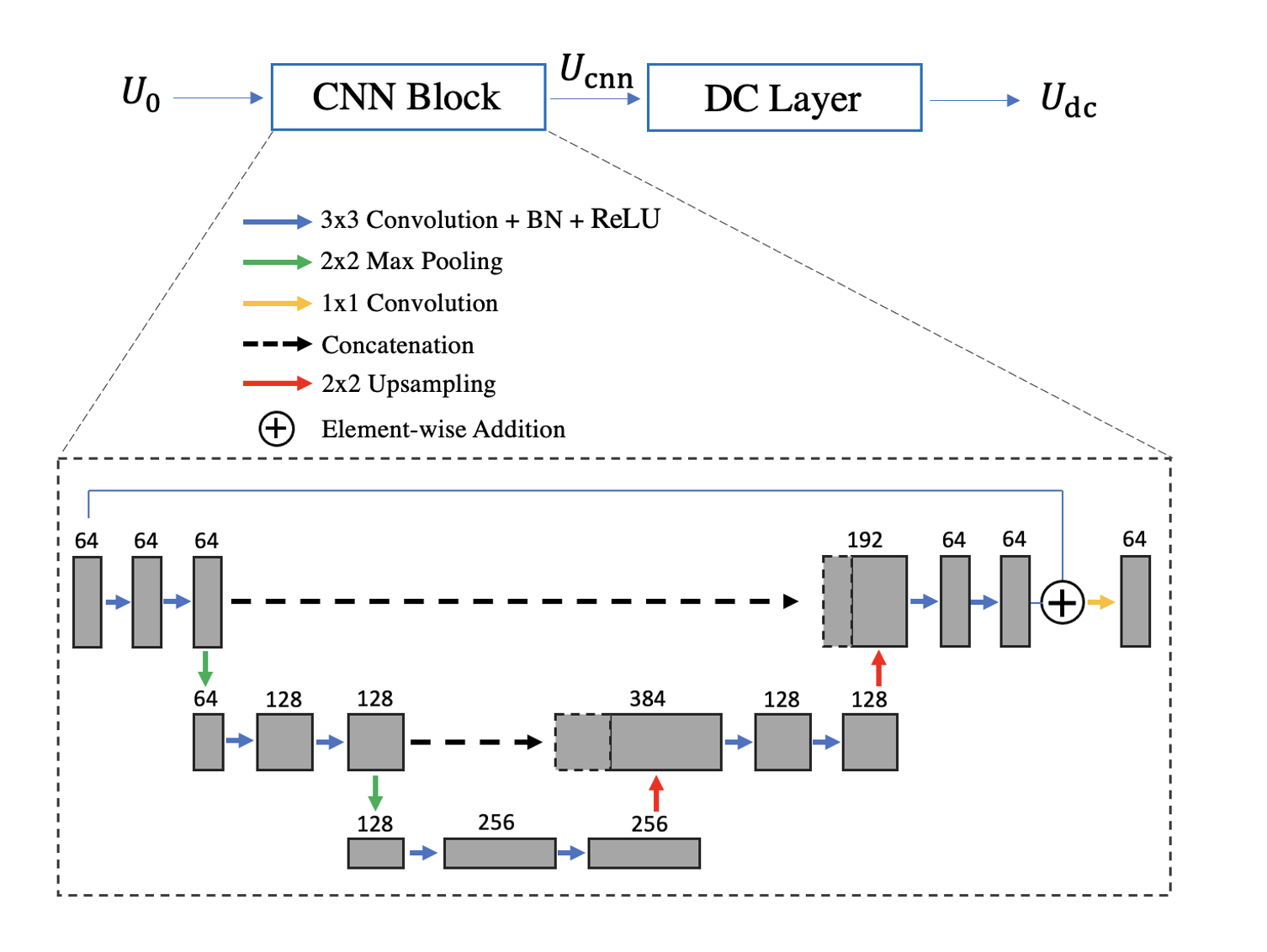
A previous study4 showed that a convolutional neural network (CNN) can quickly reconstruct $$$\mathbf{U}$$$ from a backprojected initial guess:$$\mathbf{U}_{\mathrm{cnn}}=CNN\left(\mathbf{U}_{0}\right),\tag{2}$$
where the network has been trained on iterative solutions to Eq. (1). Here, we also add a gradient descent DC layer5,6 with a preconditioner to compensate the ill-conditioning of the non-Cartesian reconstruction problem:$$\mathbf{U}_{\mathrm{dc}}=\mathbf{U}_{\mathrm{cnn}}-\alpha \mathbf{S}^{\dagger}\mathbf{P}\left[E_\mathit{\Phi}^{*}E_\mathit{\Phi}\left(\mathbf{S}\mathbf{U}_{\mathrm{cnn}}\right)-E_\mathit{\Phi}^{*}(\mathbf{b})\right]\tag{3}$$
$$E_\mathit{\Phi}(\mathbf{Y})=\mathit\Omega\left(\mathit\Phi\times_{1}\mathbf{F}_{\mathrm{NU}}\mathbf{Y}\right)\tag{4}$$
where $$$\alpha$$$ is the step-size, $$$E_\mathit{\Phi}$$$ is the encoding matrix for each channel, and $$$\mathbf{P}$$$ is the preconditioner.
Methods
Network implementation:The proposed network (Figure 1) consists of a CNN block (U-Net) and a PGD-DC layer, both of which operate entirely within a low-dimensional subspace spanned by $$$\it{\Phi}$$$. The U-Net was pretrained on single-slice data only with iteratively-reconstructed labels. The DC layer was added during validation (to determine $$$\alpha$$$) and testing, for both single-slice and SMS data.Single-slice dataset: A total of 123 60-sec single-slice radial T1 CMR multitasking datasets7 were collected from Siemens 3T scanners (Verio, mMR Biograph, and Vida). We used a 96:12:15 training:validation:testing split.
SMS dataset: A total of five 120-sec radial SMS T1 CMR multitasking datasets (basal, mid, and apical slices) with a CAIPIRINHA-type8 phase modulation pattern were collected from Siemens 3T scanners. One dataset was used for validation and four for testing.
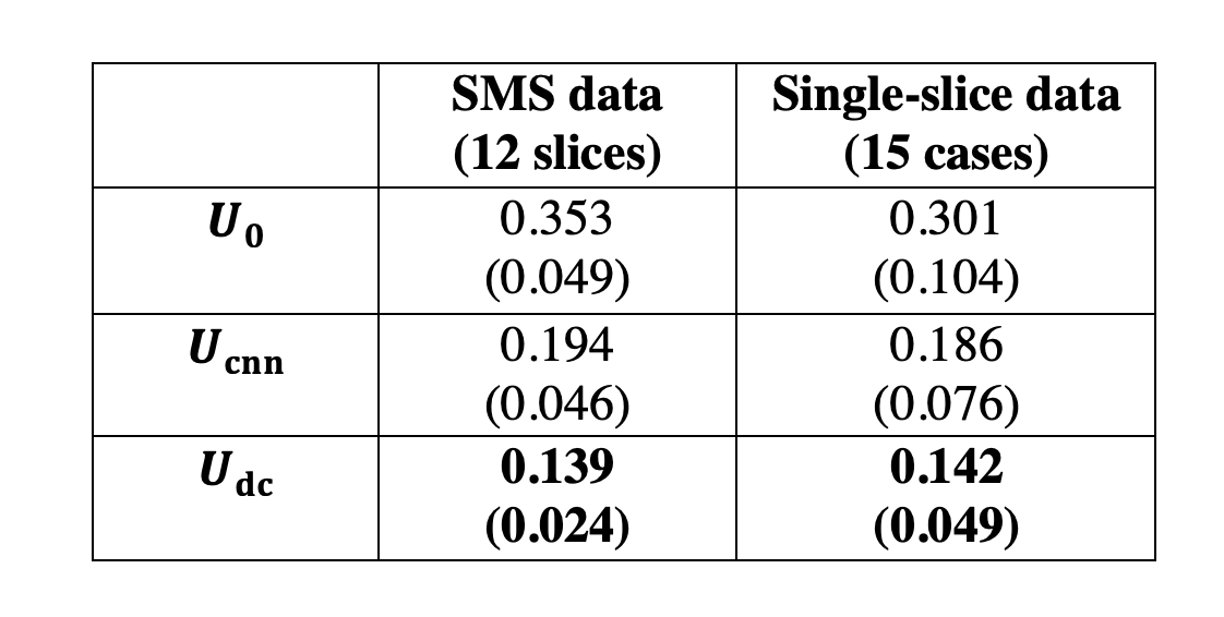
Evaluation methods: For both single-slice and SMS testing data, we compared $$$\mathbf{U}_{\mathrm{cnn}}$$$ and $$$\mathbf{U}_{\mathrm{dc}}$$$ against iteratively-reconstructed references. For spatial factors, NRMSE was compared. Paired t-tests compared error between $$$\mathbf{U}_{\mathrm{cnn}}$$$ and $$$\mathbf{U}_{\mathrm{dc}}$$$; unpaired t-tests compared single-slice and SMS NRMSEs. For dynamic images, we evaluated PSNR, SSIM and NRMSE of T1-weighted images at dark-blood contrast over the whole cardiac cycle (20 frames) at the end-expiration (EE) respiratory phase. Accuracy and precision of EE, end-diastolic septal T1 were compared against the iteratively-reconstructed T1 values using Bland-Altman plots.
Results
For single-slice data, reconstruction times were 10min for iterative reconstruction, 1sec for $$$\mathbf{U}_{\mathrm{cnn}}$$$, and 5sec total for $$$\mathbf{U}_{\mathrm{dc}}$$$. For SMS data, reconstruction times were 28min for iterative reconstruction, 2sec for $$$\mathbf{U}_{\mathrm{cnn}}$$$, and 38sec total for $$$\mathbf{U}_{\mathrm{dc}}$$$. All the reconstruction was tested on one Nvidia Titan RTX GPU.Figure 2 shows spatial factor NRMSE in the testing sets. For both SMS and single-slice data, the CNN block significantly reduced NRMSE (p<0.001) versus $$$\mathbf{U}_{\mathrm{0}}$$$, and the DC layer further reduced NRMSE (p<0.001) versus $$$\mathbf{U}_{\mathrm{cnn}}$$$. NRMSE of $$$\mathbf{U}_{\mathrm{cnn}}$$$ was not significantly different for SMS versus single-slice data (p=0.75); nor was the NRMSE of $$$\mathbf{U}_{\mathrm{dc}}$$$ for SMS versus single-slice (p=0.85).
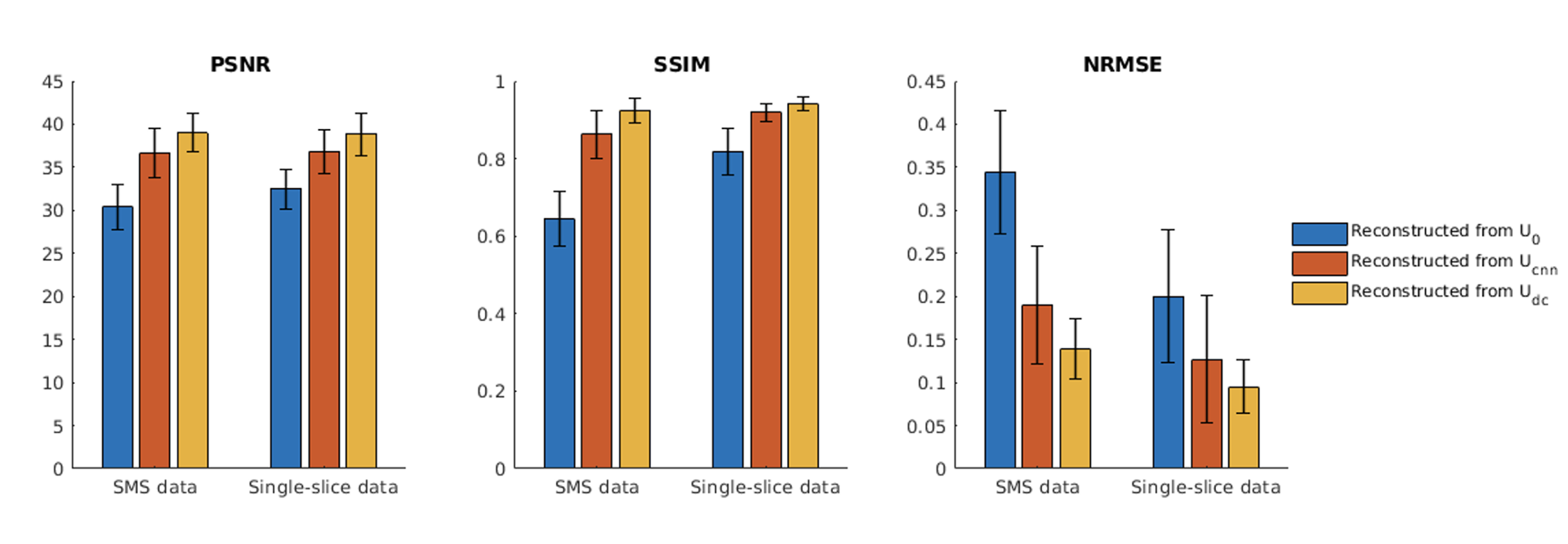
Figure 3 shows the PSNR, SSIM and NRMSE of reconstructed dynamic images. Again, the CNN improved the initial guess, and the DC layer further improved the reconstruction, for both SMS and single-slice data.
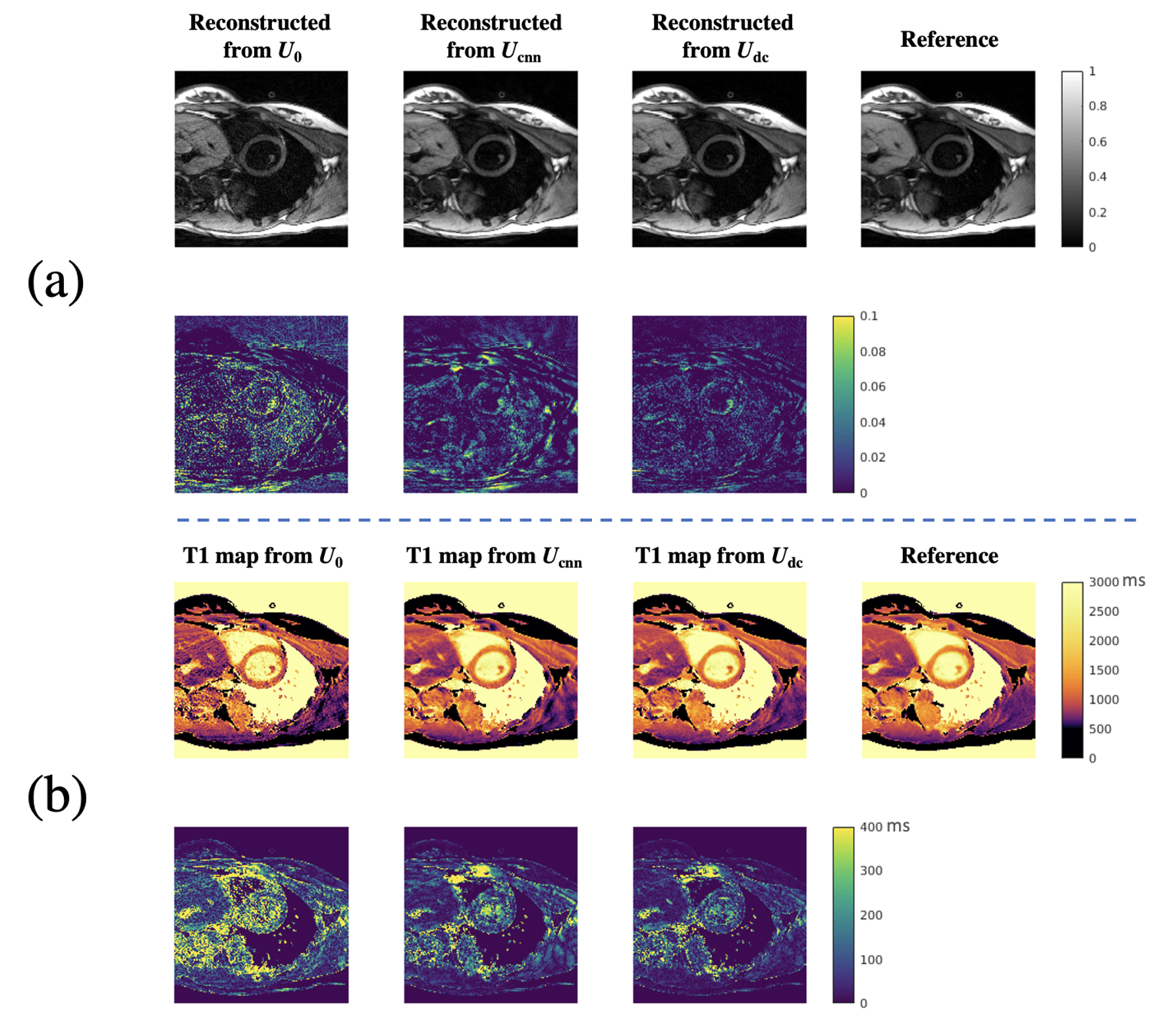
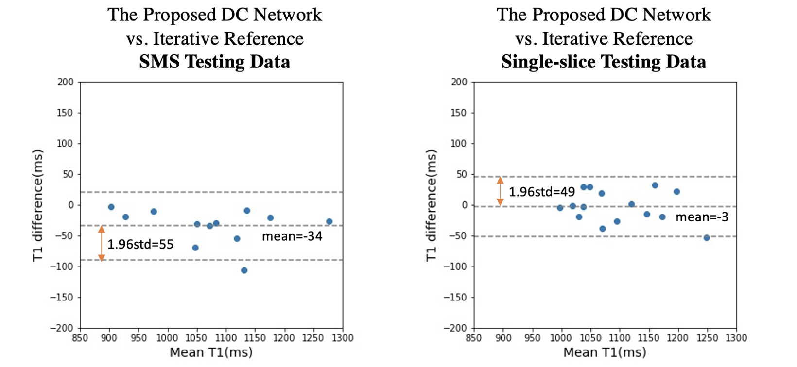
Figure 4 shows an example testing slice comparing deep learning and iteratively-reconstructed SMS images and T1 maps. Visual quality is consistent with the results in Figure 3. Figure 5 shows the Bland-Altman plots for average T1 values in the left-ventricular myocardium, for both SMS and single-slice testing data. SMS T1 values show a small (–34ms) but statistically significant bias (p=0.002) between deep learning and iterative reconstructions, but comparable precision (limits-of-agreement=±55ms) as the single-slice T1 results (limits-of-agreement=±49ms).
Discussion
Although the reconstruction network was entirely trained on single-slice data, network performance was not significantly different between SMS and single-slice testing data for weighted images. T1 precision was comparable between SMS and single-slice data, but SMS showed a small bias. It may be possible to improve T1 accuracy by incorporating small amounts of SMS training data, as will be explored in future work.Conclusion
DC deep subspace transfer learning is feasible by training on single-slice data and directly applying the network to SMS image reconstruction. Even without any SMS training data, the proposed method accelerated SMS reconstruction by >40x, producing similar NRMSE to single-slice reconstruction, and producing comparably precise T1 maps. This implies that training on one multitasking variation is transferrable to other multitasking variations, reducing the need for new training data.Acknowledgements
This work was supported by NIH grants R01 EB028146 and R01 HL156818.References
1. Christodoulou AG, Shaw JL, Nguyen C, et al. Magnetic resonance multitasking for motion-resolved quantitative cardiovascular imaging. Nature Biomed Eng. 2018;2(4):215-226.
2. Mao X, Lee H-L, Ma S, et al. Simultaneous Multi-slice Cardiac MR Multitasking for Motion-Resolved, Non-ECG, Free-Breathing Joint T1-T2 Mapping. Proc Int Soc Magn Reson Med. 2021.
3. Liu Q, Zheng Y, Lyu J, et al. Multiband Multitasking for Cardiac T1 Mapping. Proc Int Soc Magn Reson Med. 2021.
4. Chen Y, Shaw JL, Xie Y, Li D, Christodoulou AG. Deep learning within a priori temporal feature spaces for large-scale dynamic MR image reconstruction: Application to 5-D cardiac MR Multitasking. Med Image Comput Comput Assist Interv. 2019:495-504.
5. Schlemper J, Caballero J, Hajnal JV, Price AN, Rueckert D. A deep cascade of convolutional neural networks for dynamic MR image reconstruction. IEEE Trans Med Imaging. 2017;37(2):491-503.
6. Aggarwal HK, Mani MP, Jacob M. MoDL: Model-based deep learning architecture for inverse problems. IEEE Trans Med Imaging. 2018;38(2):394-405.
7. Shaw JL, Yang Q, Zhou Z, et al. Free-breathing, non-ECG, continuous myocardial T1 mapping with cardiovascular magnetic resonance multitasking. Magn Reson Med. 2019;81(4):2450-2463.
8. Breuer FA, Blaimer M, Heidemann RM, Mueller MF, Griswold MA, Jakob PM. Controlled aliasing in parallel imaging results in higher acceleration (CAIPIRINHA) for multi‐slice imaging. Magn Reson Med. 2005;53(3):684-691.
Figures