1738
Power Laws for Neurovascular Coupling between Cerebral Blood Flow and Oxygen Metabolism1National Institute of Mental Health, National Institutes of Health, Bethesda, MD, United States, 2University of Nottingham Medical School, School of Life Sciences, Nottingham, United Kingdom
Synopsis
We previously developed (CMRO2/CMRO20)=(CBF/CBF0)(1-α/β)(1-1/β)as special power relation (SPR) for brain activation. In this work, based on different perspective of SPR, we derive that functional activity induces general power relation (GPR) (CMRO2/CMRO20)=(CBF/CBF0)α/β. When α=0.38,β=1.5, both powers (SPR and GPR) are calculated to be 0.25,which is approximately equivalent to inverse of conventional coupling constant of 4. By equalizing two powers, the relationship of α and β parameters can be established. We also show that any coupling pairs between changes of CMRO2,CBF,CBV and OEF can be reduced into power laws. Finally, we propose the power law for quantification CMRO2 changes during CO2 calibration.
Introduction:
Neurovascular couplings of local oxygen extraction fraction (OEF) and cerebral metabolic rate of oxygen (CMRO2) with blood flow or volume (CBF or CBV) are key indicators in brain function1. A generally accepted model relating changes of CMRO2 with BOLD signal is Davis model2. For M parameter determination in Davis model, it was assumed that 5% CO2 hypercapnia might not change CMRO2. Several previous works challenged this assumption both in non-invasive and invasive measures3,4, suggesting decreased CMRO2 during hypercapnia. In addition, determination of α and β parameters used in Davis model is another controversial issue5,6.In this work, first, we derived general power law relations (GPR) of CMRO2 and CBF; Second, we show that any coupling pairs between changes of CMRO2, CBF, CBV and OEF can be reduced into power laws; Third we establish relationship of α and β parameters. Fourth, we propose the power law equation for quantification CMRO2 changes during CO2 calibration. In our approach, α and β are treated as variables. More importantly, we assume the negative changes of CMRO2 during the CO2 calibration.
Theory and Methods
We denote δ as operator for percentage change. For example, BOLD signal percentage is δ(STE)=ΔS/S0=S/S0 -1, S and S0 refer to activation and resting state, respectively.- General power relation (GPR)
Davis equations are known as Eq.1_a and Eq.1_b:
$$\frac{CMRO2}{CMRO2_{0}}=\left(1-\frac{\delta(S_{TE})}{M}\right)^\frac{1}{\beta}\left({\frac{CBF}{CBF_{0}}}\right)^\left(1-\frac{\alpha}{\beta}\right),\ \left(Eq.1\_a\right), or\ \delta(S_{TE})=M\left(1-\left(\frac{CBV}{CBV_{0}}\right)\left(\frac{OEF}{OEF_{0}}\right)^\beta\right),\ \left(Eq.1\_b\right),$$
where δ(STE) is BOLD, α, β are constants; M represents maximum BOLD response. Eq.1_a and Eq.1_b are equivalent due to Grubb’s rule of Eq.2_a and Fick’s law of Eq.2_b.
$$\left(\frac{CBV}{CBV_{0}}\right)=\left(\frac{CBF}{CBF_{0}}\right)^\alpha,\ \left(Eq.2\_a\right),\ \left(\frac{CMRO2}{CMRO2_{0}}\right)=\left(\frac{CBF}{CBF_{0}}\right)\left(\frac{OEF}{OEF_{0}}\right),\ \left(Eq.2\_b\right),$$
Due to the power relation of CBF and CMRO2 suggested by our previous work7, alternatively, we may hypothetically assign that
$$\left(\frac{CMRO2}{CMRO2_{0}}\right)=\left(\frac{CBF}{CBF_{0}}\right)^{p_{x}},\ \left(Eq.3\right),$$
where px is a power constant to be determined. By introducing Eq.3 into Eq.2_a and Eq.2_b, and subsequently with Eq.1_b, we reach to Eq.4.
$$\frac{CMRO2}{CMRO2_{0}}=\left(1-\frac{\delta(S_{TE})}{M}\right)^\frac{p_{x}}{\alpha}\left(\frac{CBF}{CBF_{0}}\right)^{(\frac{p_{x}}{\alpha})(\beta-\beta{p_{x}})},\ \left(Eq.4\right),$$
By matching all powers of Eq.4 with the powers in Davis Eq.1_a, the unknown power of px can be determined to be α/β. Consequently, we reach to GPR relation Eq.5.
$$\frac{CMRO2}{CMRO2_{0}} =\left(\frac{CBF}{CBF_{0}}\right)^ \frac{\alpha}{\beta},\ \left(Eq.5\right),$$ - Special power relations (SPR)7
We previously showed that
$$\delta(S_{TE})=M\left(1-\left(\frac{CBF}{CBF_{0}}\right)^\left(\frac{\alpha}{\beta}-1\right)\right), \ \left(Eq.6\_a\right),\ and,\ \frac{CMRO2}{CMRO2_{0}} =\left(\frac{CBF}{CBF_{0}}\right)^ {(1-\frac{\alpha}{\beta})(1-\frac{1}{\beta})} \ \left(Eq.6\_b\right),$$
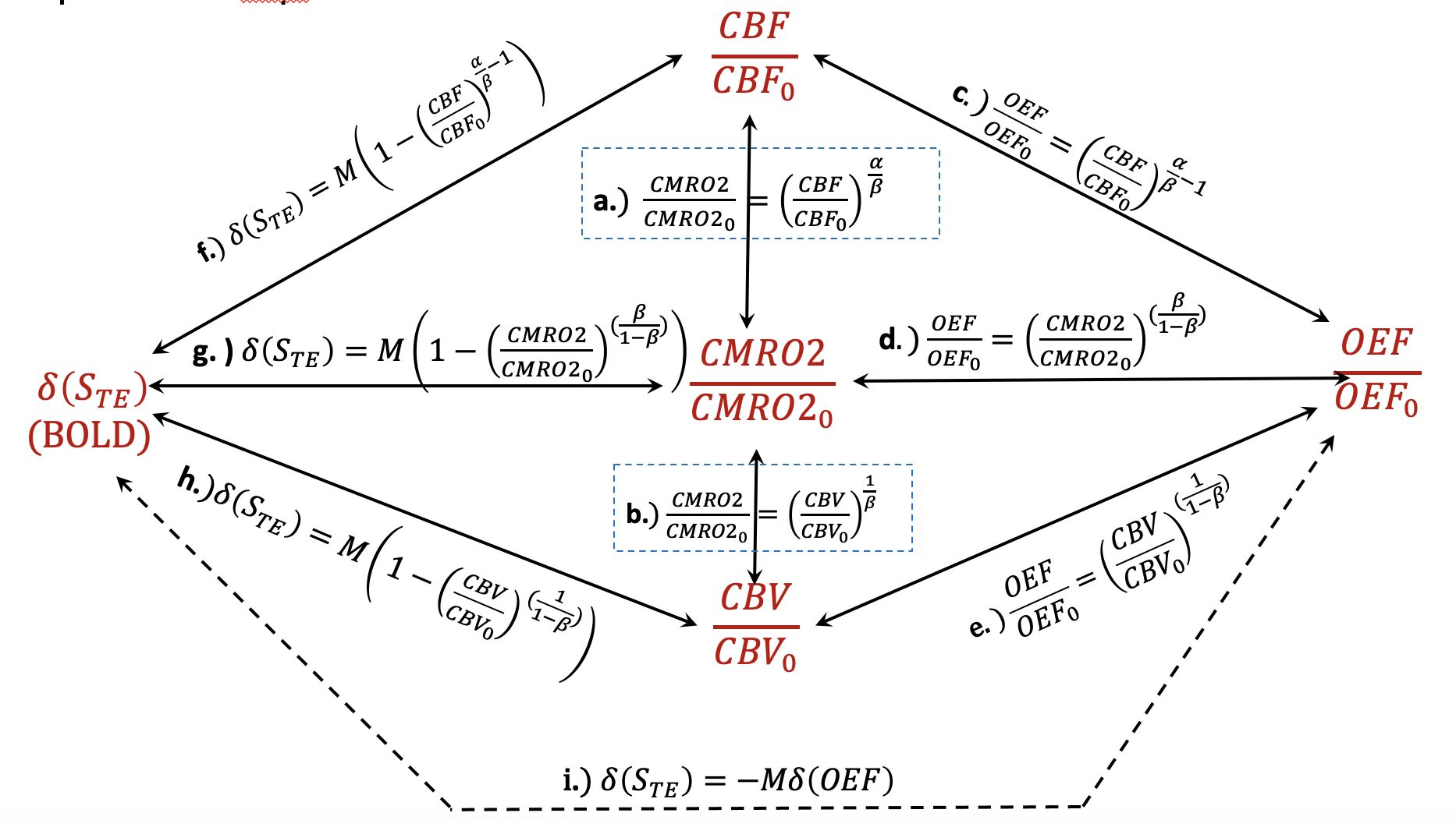
Relying on Eq.5, Eq6_a, Eq.2_b and Eq.1_b, we can show in Fig.1 all the special power relations (SPR). - Relationship of α and β
GPR Eq.5 and SPR Eq.6_b both were derived from Fick’ law and Davis model. They must be compatible to each other, which was supported by the fact that when introduced generally accepted values of α=0.38 and β=1.5, both are equal to 0.25. Thus, the powers of GPR and SPR are equal, after rearrangement, as Eq.7.
$$\frac{\alpha}{\beta} =\frac{1-\beta}{1-2\beta} \ \left(Eq.7\right),$$ - Power law for quantification CMRO2 change during CO2 hypercapnia
In CO2 hypercapnia, we assume the changes of CMRO2 and CBF are still complied with Eq.5 and Eq.6_a, except that the CMRO2 is decreased when CBF is increased. By replacing δ(CMRO2) in CMRO2/CMRO20=δ(CMRO2)+1 with negative sign, we can have CMRO2/CMRO20=1-δ(CMRO2), which is equivalent to (CMRO2/CMRO20)-1. Therefore, during CO2 calibration, $$\delta(S_{TE})_H=M\left(1-\left(\frac{CBF}{CBF_{0}}\right)_H^\left(-\frac{\alpha}{\beta}-1\right)\right), \ \left(Eq.8\_a\right),\ and,\ \left(\frac{CMRO2}{CMRO2_{0}}\right)_H =\left(\frac{CBF}{CBF_{0}}\right)_H^ \left(-\frac{\alpha}{\beta}\right) \ \left(Eq.8\_b\right),$$ where H refers to the hypercapnia. Comparing Eq.8_a with Eq.6_a, the power of component of (CBF/CBF0)Hα/βwas replaced with negative power sign because it reflexes to the negative changes of CMRO2. The power of (CBF/CBF0)H in the denominator remains the same positive sign because it represents the positive change of CBF. - Calculating the ratio of α/β
Dividing Eq.6_a with Eq.8_a yields Eq.9. $$\frac{\delta(S_{TE})_F}{\delta(S_{TE})_H}=\frac{\left(1-\left(\frac{CBF}{CBF_{0}}\right)_F^\left(\frac{\alpha}{\beta}-1\right)\right)}{\left(1-\left(\frac{CBF}{CBF_{0}}\right)_H^\left(-\frac{\alpha}{\beta}-1\right)\right)},\ \left(-1\leq{\frac{\alpha}{\beta}}\leq1\right),\ \left(Eq.9\right),$$ where H and F refers to the hypercapnia and functional data, respectively. Applying Taylor expansion on Eq. 9, we may prove α/β is between -1 and 1.
Results and Discussion
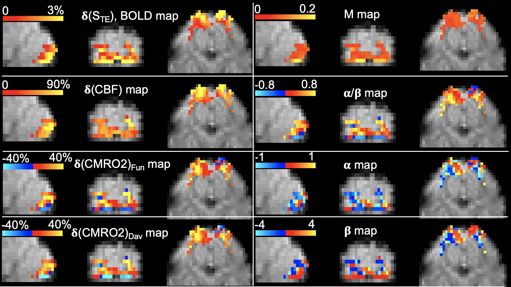
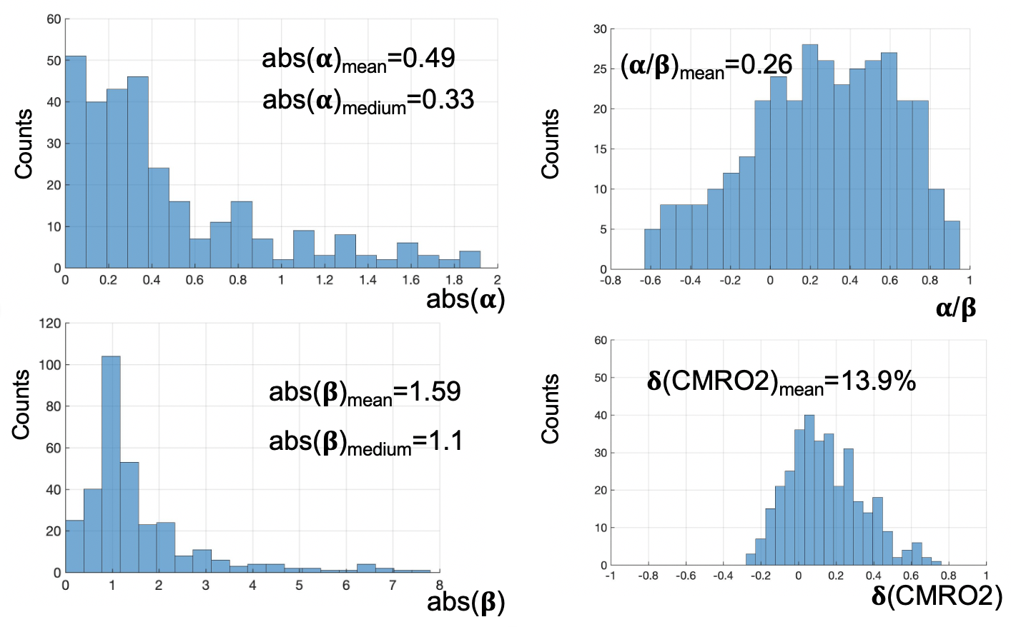
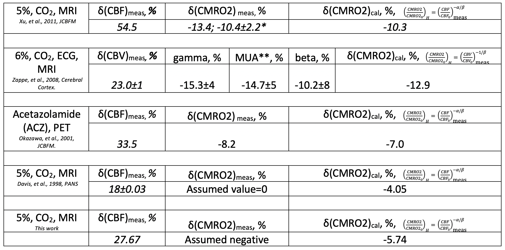
Results across 11 subjects were shown in Table.1. The averages of α/β is 0.252, which is approximately equal to inverse notion of conventional coupling constant of 4, when changes of CBF and CMRO2 are small. The averaged α=0.38 and β=1.51 across 11 subjects, (calculated by inputting α/β=0.252 into Eq. 7), agree with the with conventional values of α=0.38 and β=1.5. The mean M value 0.088 from this approach agrees with the M value of 0.089 from Davis approach. Varieties of maps and histograms extracted from one subject were shown in Fig.2 and Fig.3, respectively. To further verify the quantification for negative change of CMRO2, in Tab. 2, we compare the measured CMRO2 changes (δ(CMRO2)meas) reported in previous studies with calculated CMRO2 changes (δ(CMRO2)cal), which was calculated by using accordingly measured CBF changes in these works. We found good agreement in CMRO2 changes between calculation and measurements, even under different vasodilation conditions, such as administration of CO2 and acetazolamide (ACZ).Acknowledgements
This work was supported by the Intramural Research Program of the National Institute of Mental Health, USA.References
1. Buxton, R. B. Interpreting oxygenation-based neuroimaging signals: the importance and the challenge of understanding brain oxygen metabolism. Front. Neuroenergetics 2, 1–16 (2010).
2. Davis, T. L., Kwong, K. K., Weisskoff, R. M. & Rosen, B. R. Calibrated functional MRI: Mapping the dynamics of oxidative metabolism. Proc. Natl. Acad. Sci. U. S. A. 95, 1834–1839 (1998).
3. Xu, F. et al. The influence of carbon dioxide on brain activity and metabolism in conscious humans. J. Cereb. Blood Flow Metab. 31, 58–67 (2011).
4. Zappe, A. C., Uludaǧ, K., Oeltermann, A., Uǧurbil, K. & Logothetis, N. K. The influence of moderate hypercapnia on neural activity in the anesthetized nonhuman primate. Cereb. Cortex (2008) doi:10.1093/cercor/bhn023.
5. Chen, J. J. & Pike, G. B. BOLD-specific cerebral blood volume and blood flow changes during neuronal activation in humans. NMR Biomed. 22, 1054–1062 (2009).
6. Gagnon, L. et al. Validation and optimization of hypercapnic-calibrated fMRI from oxygen-sensitive two-photon microscopy. Philos. Trans. R. Soc. B Biol. Sci. 371, (2016).
7. Li, L., Marrett, S., Derbyshire, A. J. & Bandettini, P. Non-calibrated Equations for Quantification of Local fMRI Signal Changes with Hemodynamic Oxygen Metabolism ( CBF and CMRO2 ). Proc. Intl. Soc. Mag. Reson. Med.(2021).
8. Blockley, N. P., Griffeth, V. E. M., Simon, A. B., Dubowitz, D. J. & Buxton, R. B. Calibrating the BOLD response without administering gases: Comparison of hypercapnia calibration with calibration using an asymmetric spin echo. Neuroimage 104, 423–429 (2015).
Figures