INTRODUCTION

Diffusion Tensor Imaging is a Magnetic Resonance Imaging method sensitive to brain microstructure and can be used clinically to investigate pathological alterations. Theoretically, 7 diffusion-weighted (DW) images are required to estimate the diffusion tensor (DT) with model fitting, but in practice it has been widely demonstrated that increasing the number of DW volumes (e.g. to 35 or 60^1,2) results in less noisy and biased DT estimates. This inevitably leads to long acquisition times limiting the DT clinical viability. The most used quantitative map obtained from the DT is fractional anisotropy (FA), which is highly sensitive to changes in tissue microstructure^3,4.
Here we investigate the possibility of reducing the number of DW volumes to dramatically reduce acquisition time, through deep learning (DL), while retaining or enhancing image quality exploiting the fact that a DL network can contribute to image quality transfer⁵. We implemented a DL network that can: 1) map from a small number of DW volumes (10) to FA; 2) take advantage of datasets with high-geometrical and DW angular resolution with corresponding high-quality FA maps for training the network, e.g using data from the Human Connectome Project (HCP)⁶; 3) tackle the generalization problem: given a network trained with a specific dataset, offer applicability to clinical datasets from different scanners without re-training; and, 4) retain sensitivity to pathology. We validated the network with unseen data from the HCP dataset and with two datasets from temporal lobe epilepsy (TLE) and multiple sclerosis (MS) studies, acquired with different protocols on different scanners.

METHODS

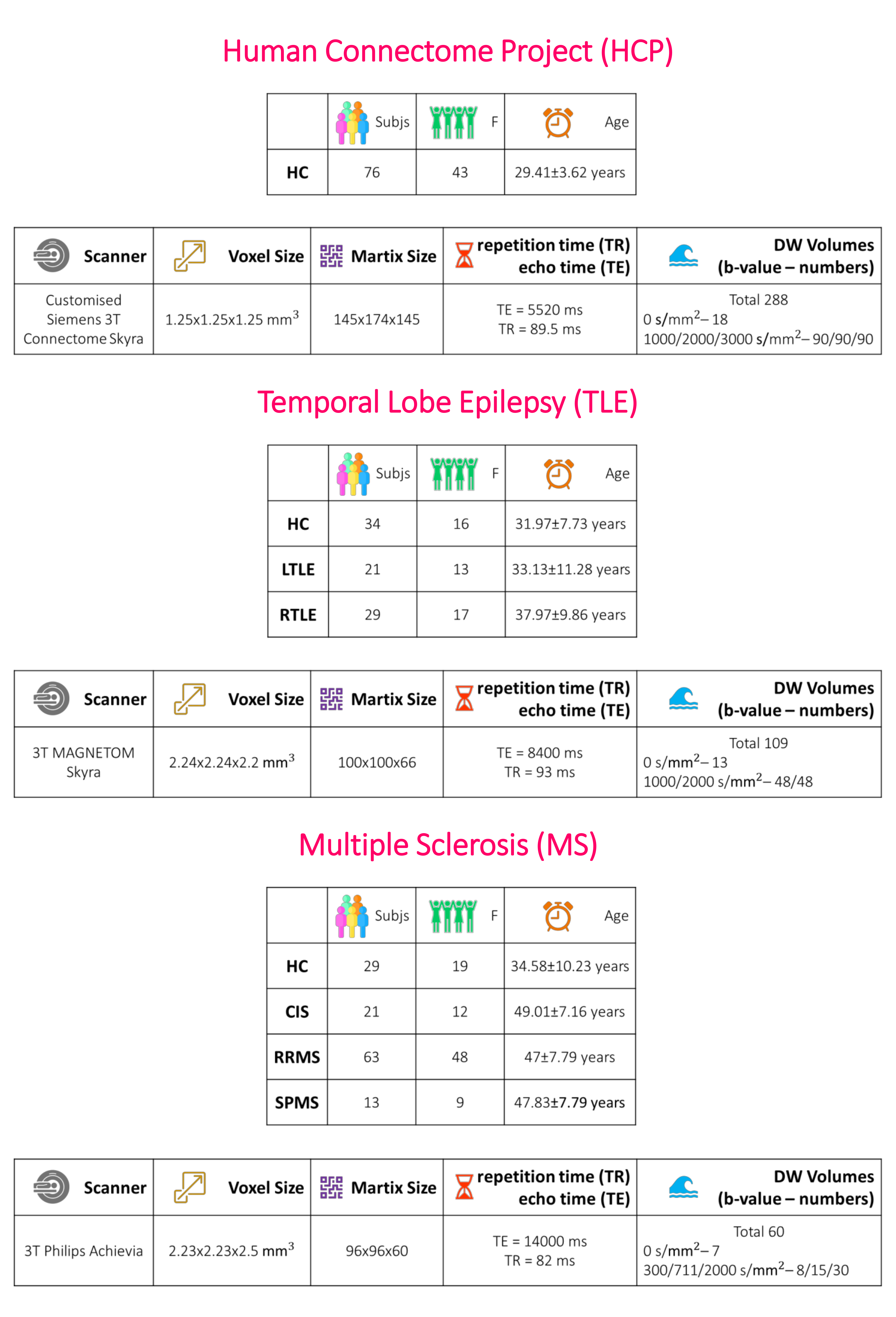
Datasets: Fig.1 shows the demographics and MRI acquisition details. A standard FA map, from DT fitting (DESIGNER⁷), was calculated considering all DW volumes for each dataset.
Data preparation: The HCP dataset included 54 subjects for training, 11 for validation and 11 for test. Standard FA maps were used as ground-truth (GT). We cropped the images to 128x160 voxels. We normalized the DWI intensity for each subject separately, considering all volumes together.
We used Camino⁸ to select subsets of b-vectors equally distributed in space, obtaining 10 different DW-subsets containing 9 volumes with b-value=1000s/mm2 to which one random volume with b-value=0 was added. We also calculated the standard FA from one subset.
Network architecture: We adapted the U-net architecture⁹: the input was one of the 10 DW subsets, where each volume was a channel, with a single output channel to FA. The loss function was the root mean square error (RMSE).
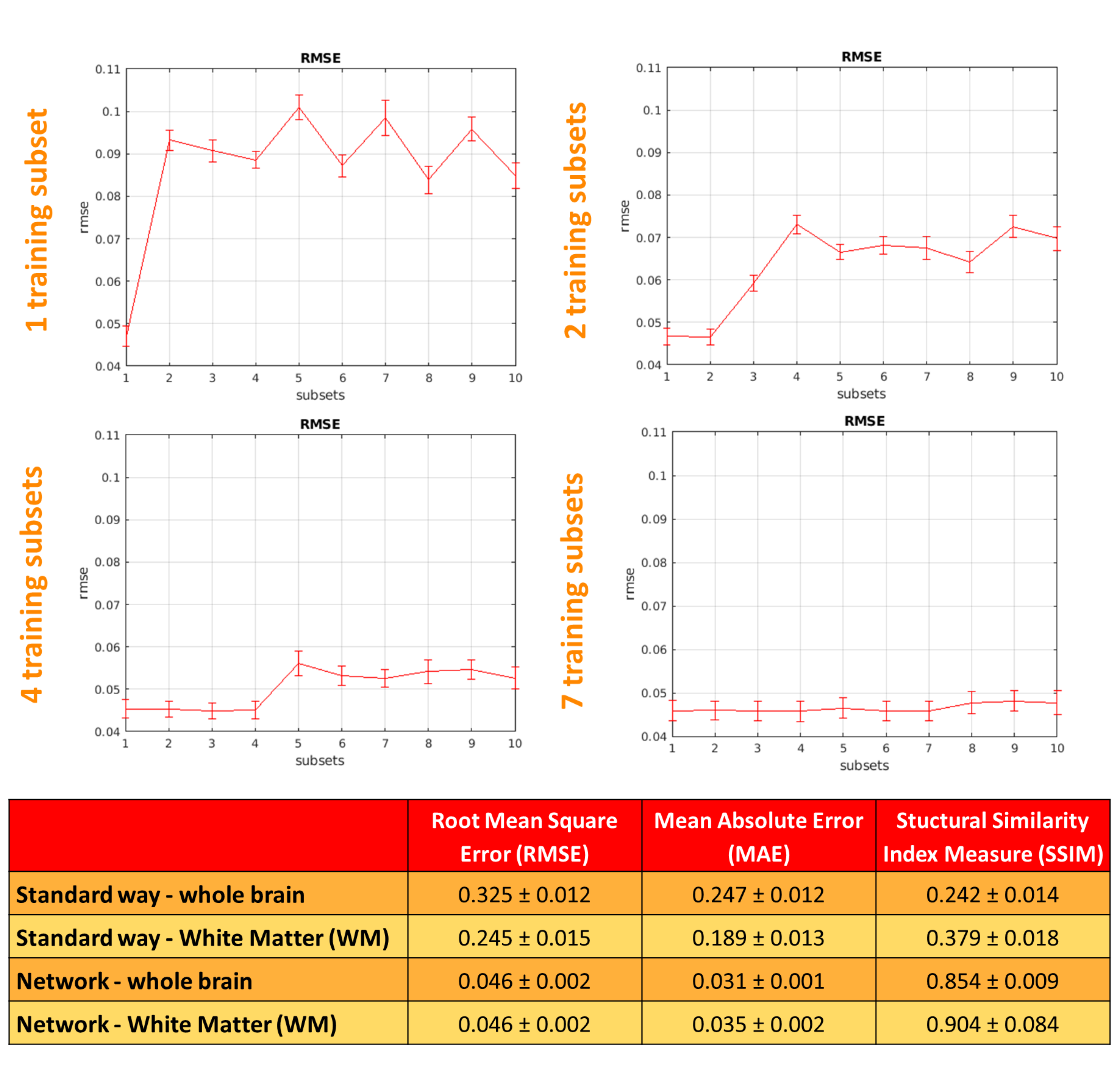
Training: The best combination of hyperparameters was the one with the lowest mean RMSE on the validation subjects. The choice of DW inputs is crucial for estimating FA: we trained the network 4 times by increasing the number of DW subsets as input (1,2,4,7) each matching the same FA (GT).
Performance assessment: RMSE, mean absolute error and structural similarity index measure¹⁰ were calculated at voxel level between the GT and the network output considering only brain voxels. To assess generalisability to unseen DW volumes combinations, each of the 4 trained networks were applied to each of the 10 DW-subsets of the test subjects. We chose the network with the most similar performance, e.g. similar RMSE, using the DW training subsets and the remaining DW subsets.
Clinical Sensitivity: Our ultimate aim was to use our network with clinical datasets, acquired with limited DW volumes and coarser resolution compared to HCP data, to maintain or improve FA quality and sensitivity to pathological changes. We used the TLE and MS datasets to evaluate network performance. Per dataset, DW data were resampled and cropped to HCP resolution, the 9 most non-collinear directions were chosen (Camino) and our network was applied.
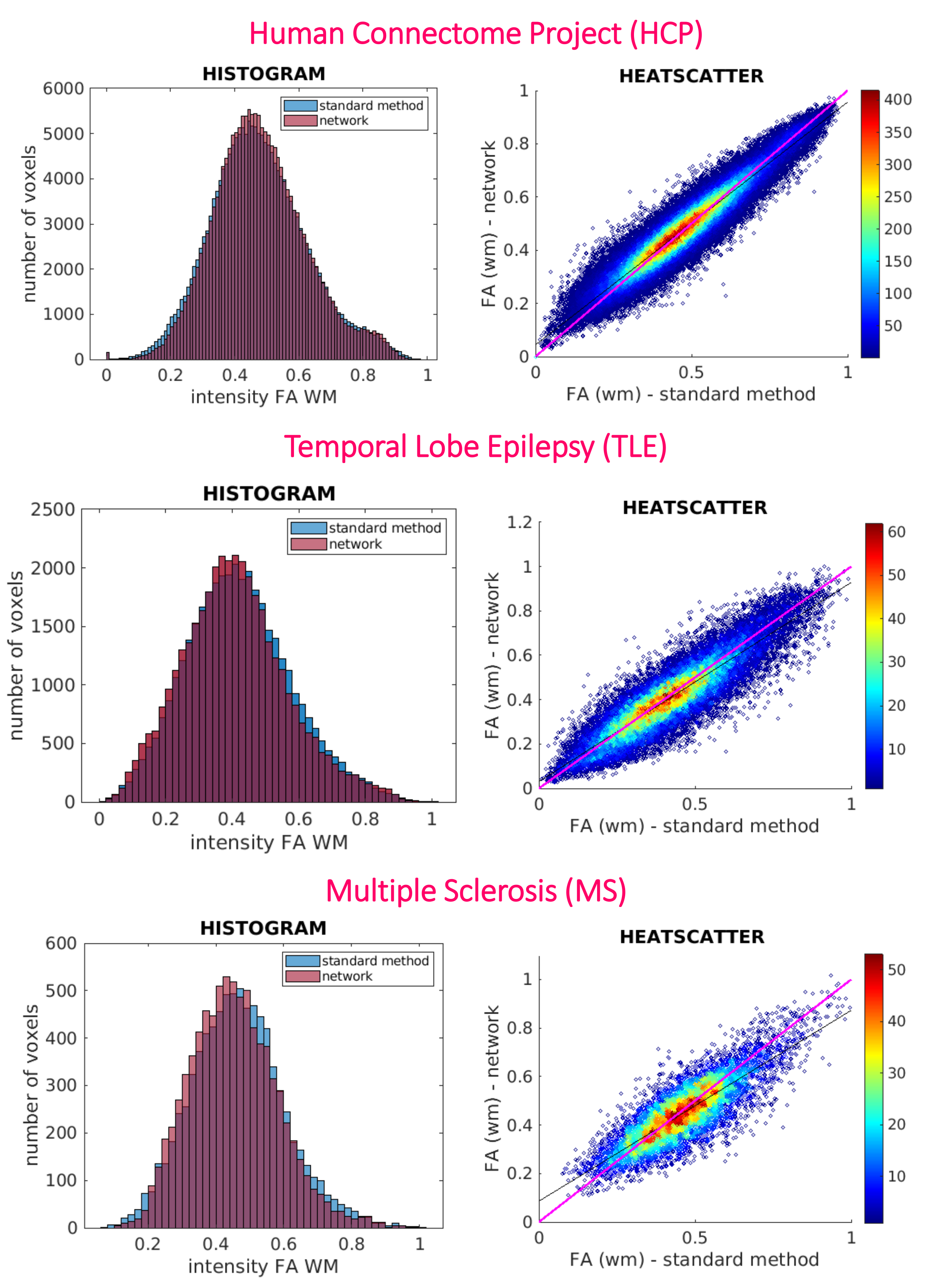
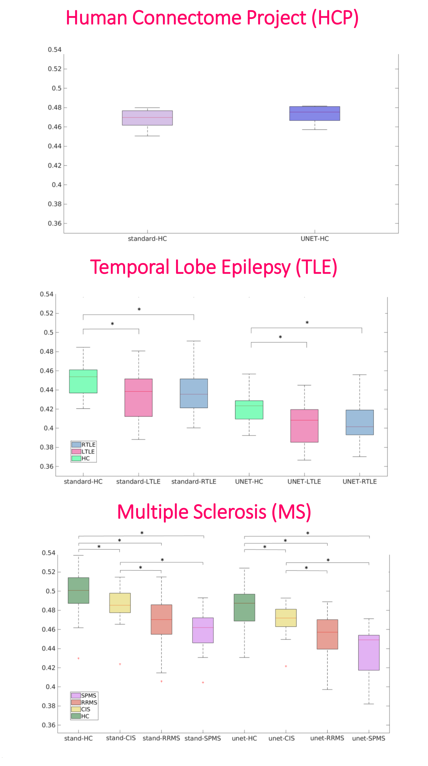
White matter (WM) quantitative assessment: WM-FA values from standard-full-DW and network-subset-DW data were compared at subject-level using histogram and heatscatter plots and at group-level using boxplot of subject’s mean WM-FA. For clinical datasets, statistics between groups verified whether biases were introduced in WM-FA when using the network-FA compared to GT.

RESULTS

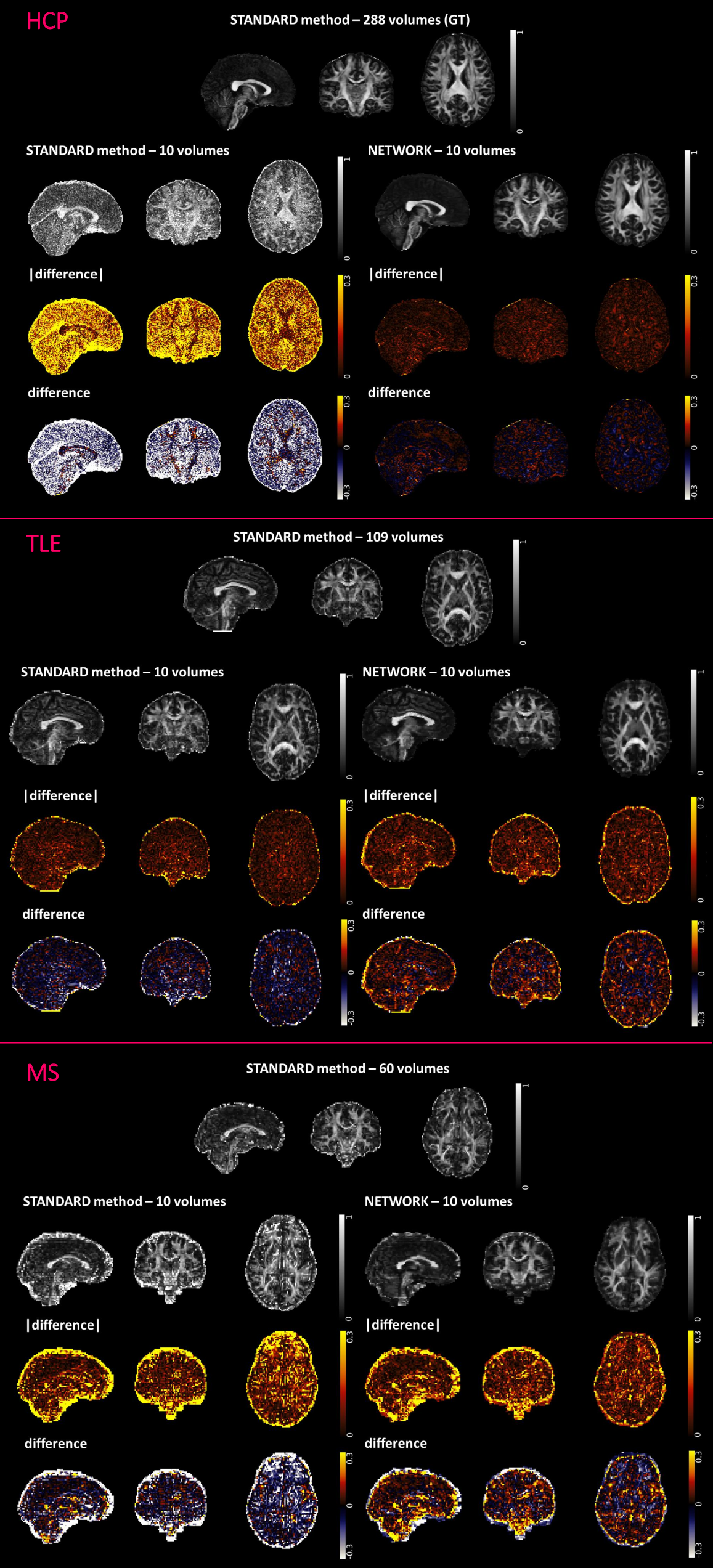
We selected the network trained with 7 DW subsets and we reported its performance metrics for the HCP test subjects (Fig.2). Fig.3 shows for each dataset each FA (standard-full-DW, standard-subset-DW, network-subset-DW). Fig.4 shows WM-FA plots in a single-subject and Fig.5 the boxplots at group-level with group differences indicated when significant.

DISCUSSION & CONCLUSIONS

We implemented a network capable of obtaining FA from a reduced set of 10 DW volumes. For HCP, the network-FA (RMSE = 0.046) was much closer to the GT than the standard-FA (DT fitting) from the same 10 DW volumes (RMSE = 0.325).
Our network maintained FA properties even on clinical data acquired on different scanners, with different DW directions and different b-values. Single-subjects FA distribution in WM voxels was maintained when using the network FA for all datasets (Fig.4).
The network FA retained properties of the standard-FA with all volumes, including sensitivity to pathology. Significant pathological differences between groups found when using the full DW dataset for standard-FA remained significant when using FA estimated by the network.
Acquiring only 10 DWI greatly reduces acquisition time and reconstruction with our network could enable the use of FA in the clinic. Future works will aim to reconstruct other DT maps of tissue microstructure in addition to FA.

Acknowledgements

This research received funding by H2020 Research and Innovation Action Grants Human Brain Project 785907 and 945539 (SGA2 and SGA3) and by the MNL Project “Local Neuronal Microcircuits” of the Centro Fermi (Rome, Italy) to FP. CGWK received funding from the UK MS Society (#77), Wings for Life (#169111), Horizon2020 (CDS-QUAMRI, #634541), BRC (#BRC704/CAP/CGW).