Introduction

Intravoxel incoherent motion (IVIM) imaging is a diffusion-weighted MR technique, which can simultaneously measure the parenchymal diffusion (D_par) and microvascular pseudo-diffusion (D_mv).¹ Recently, the presence of a third, intermediate diffusion component (D_int) was revealed, which was suggested to represent interstitial fluid (ISF) within the parenchyma.^2,3 D_int was furthermore found to be related to cerebral small vessel disease (cSVD) markers, such as white matter hyperintensities (WMH).² However, with current fitting techniques, extracting accurate voxel-wise measures for the three diffusion components is extremely hard due to the strong influence of noise. Recently, Troelstra et al.⁴ showed that fitting a tri-exponential IVIM model using an unsupervised physics-informed neural network (PI-NN) resulted in more robust voxel-wise IVIM parameters compared to the conventional least squares (LSQ) method in the liver.
In this study, we have adapted the three-component PI-NN to estimate the cerebral diffusion components (D_par, D_int and D_mv). We aimed to assess the performance of our PI-NN compared to conventional LSQ in terms of test-retest repeatability (using in-vivo data of patients with cerebrovascular disease) and accuracy (using simulations).

Methods

In-vivo data: Sixteen patients with cerebrovascular disease (cSVD (n=11) and cortical stroke (n=5)) underwent brain MRI twice on separate days (Philips Achieva 3.0T). IVIM images were acquired with diffusion sensitization in three orthogonal directions, and included an inversion pulse for cerebrospinal fluid suppression (single-shot spin-echo echo-planar-imaging (EPI), 2.4 mm cubic voxel size, b-values: 0,5,7,10,15,20,30,40,50,60,100,200,400,700, and 1000 s/mm²). Additionally, T₂-weighted FLAIR and T₁-weighted images were acquired for anatomical reference.
Image analysis: The IVIM images were corrected for head displacement, EPI and eddy current distortions (ExploreDTI). The three-component cerebral IVIM model, accounting for the inversion recovery, was described as:²

\begin{equation}S(b)=S(0)*[\frac{(1-f_{mv}-f_{int})E_{1,par}E_{2,par}e^{-bD_{par}}+f_{int}E_{1,int}E_{2,int}e^{-bD_{int}}+f_{mv}E_{1,mv}E_{2,mv}e^{-bD_{mv}}}{(1-f_{mv}-f_{int})E_{1,par}E_{2,par}+f_{int}E_{1,int}E_{2,int}+f_{mv}E_{1,mv}E_{2,mv}}\;\;\;\;\;\;\;\;\;[Eq.\;1]\end{equation}\begin{equation}with\;E_{1,k}=(1-2e^{-\frac{TI}{T_{1,k}}}+e^{-\frac{TR}{T_{1,k}}})\;for\;k=par,int;\;E_{1,mv}=(1-e^{-\frac{TR}{T_{1,blood}}});\;E_{2,k}=(e^{-\frac{TE}{T_{2,k}}})\;for\;k=par,int,mv)\end{equation}

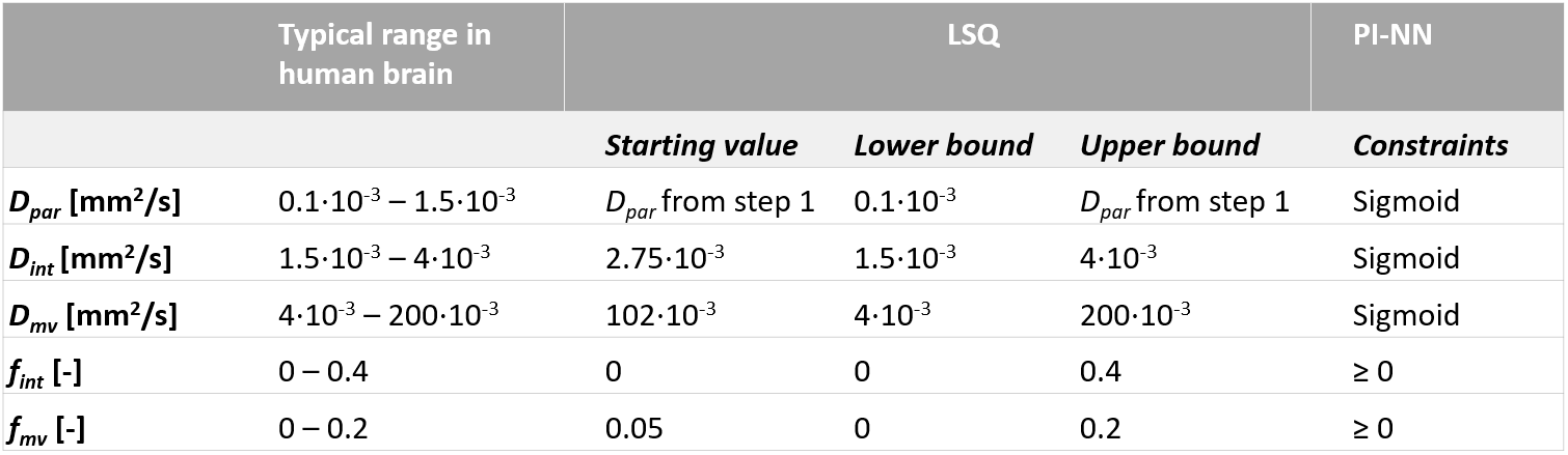
Here, f_mv and f_int are the volume fractions of the D_mv and D_int components, respectively. Both LSQ and PI-NN fitting approaches were applied to the Trace images in a voxel-wise manner. For the LSQ approach, a two-step Levenberg-Marquardt algorithm was used with lower and upper bounds equal to typical ranges found with IVIM in the human brain (Table 1).² For the PI-NN approach, the hyperparameters and training features were based on a previous study with some small adjustments to make it suitable for brain data.⁵ For example, the loss function was changed according to Equation 1. The diffusivity parameters were constrained by a sigmoid function, and the fractions were constrained to be positive (Table 1). To mitigate the problem of variable results due to repeated training, we trained 20 instances of the PI-NN model on all brain voxels in the in-vivo dataset and averaged the corresponding predictions.⁵ The white matter (WM) and cortical gray matter (cGM) were automatically segmented from the T₁-weighted images using Freesurfer, whereas WMH were semi-automatically segmented from the FLAIR images.⁶
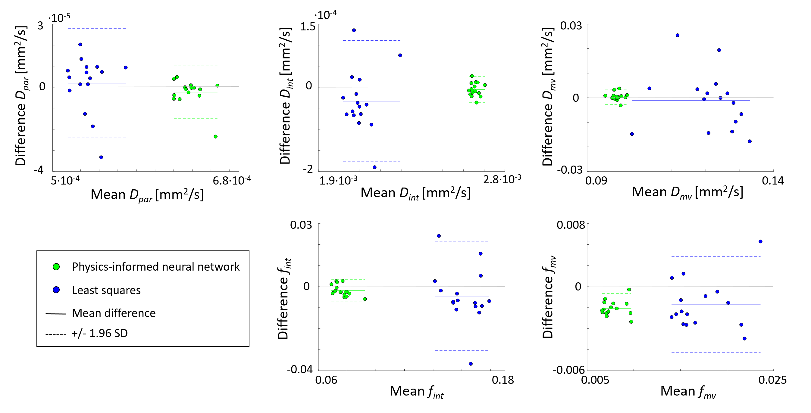
Statistical analysis: After voxel-wise fitting, the IVIM parameters were averaged over all brain voxels per subject scan. As a measure of precision, the test-retest repeatability of these IVIM parameters was quantified using the within-subject coefficient of variation (CV) and the intraclass correlation coefficient (ICC) (calculated using a one-way random model).⁷ Statistical difference between the CVs obtained with LSQ and PINN was tested with a paired Wilcoxon signed-rank test. Furthermore, Bland-Altman plots were created to visually compare the effect of PI-NN and LSQ on the repeatability.
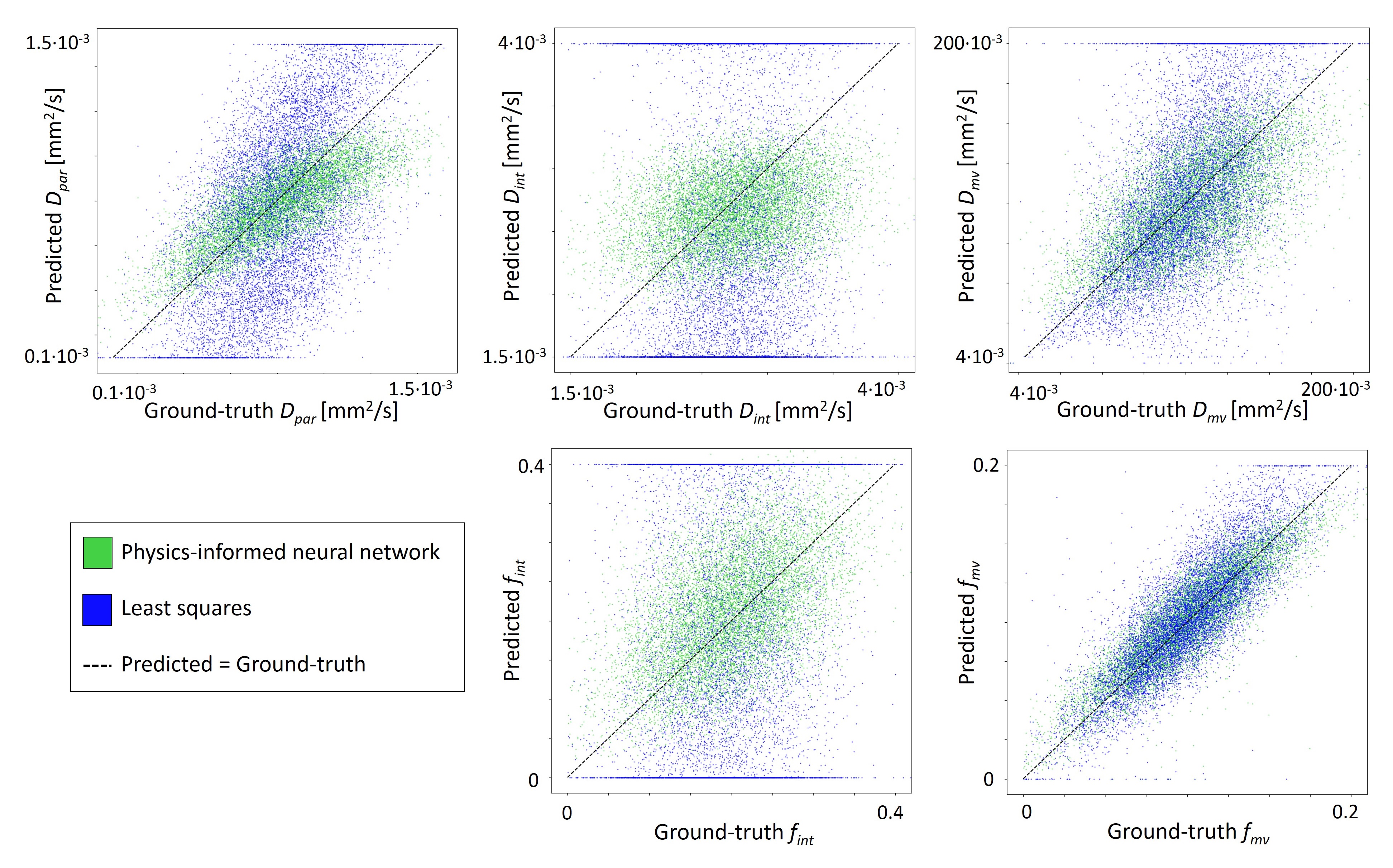
Simulated data: 10.000 IVIM signal curves were generated using Equation 1, while randomly sampling the five IVIM parameters from a Gaussian distribution (97.7% within the ranges given in Table 1). Gaussian noise was added, similar to the noise level in our in-vivo data (signal-to-noise ratio at b=0 s/mm² was 35).⁸ An ensemble of 20 PI-NN models was trained on 1.000.000 noisy IVIM signal decay curves. Subsequently, the PI-NN and LSQ fitting approaches were applied to the synthesized curves to predict the IVIM parameters. The accuracy of both methods was quantified with the normalized root-mean-square error (NRMSE) between all ground-truth and predicted IVIM parameters.

Results

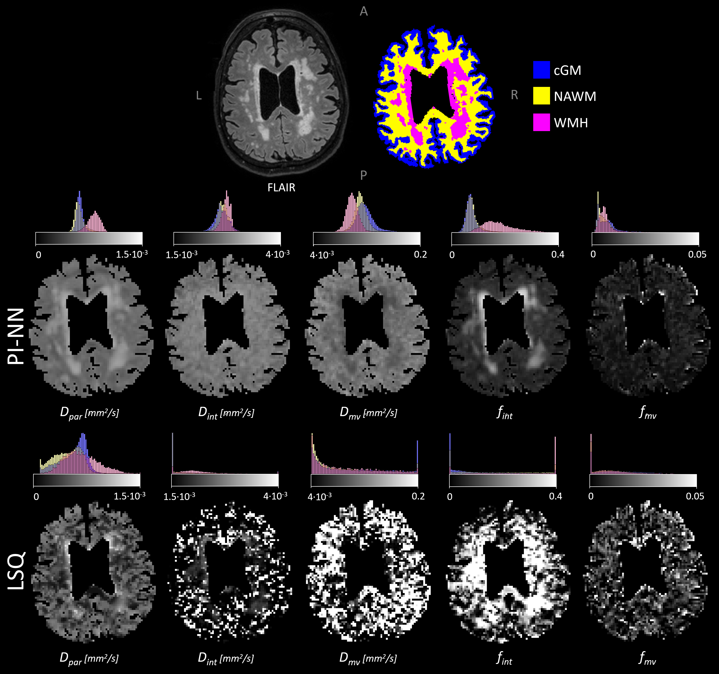
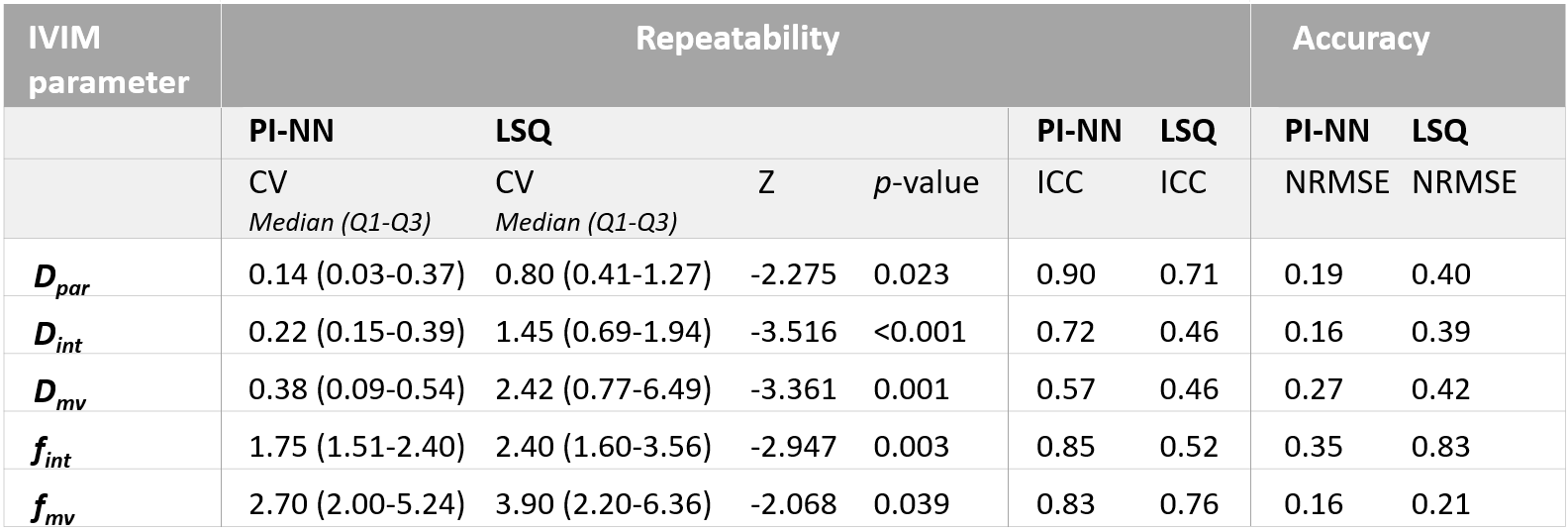
In-vivo data: The IVIM parameter maps obtained with the PI-NN and LSQ fitting approach of a representative cSVD patient are shown in Figure 1. The PI-NN maps appear smoother, while still retaining reasonable contrast between different tissue types (e.g. higher D_par, higher f_int and lower D_mv in WMH compared to normal-appearing WM). The PI-NN method was more precise than the LSQ, as it showed higher test-retest repeatability in terms of lower CV and higher ICC values (Table 2). This was also illustrated by the smaller differences between the test-retest of the PI-NN measurements using Bland-Altman plots (Figure 2).
Simulated data: Figure 3 shows scatterplots of the ground-truth and predicted IVIM parameters. Overall, the PI-NN was more accurate as it had a lower NRMSE than the LSQ (Table 2).

Discussion & Conclusion

In this study, we demonstrated the applicability of a PI-NN for three-component cerebral IVIM fitting in patients with cerebrovascular disease. The PI-NN method resulted in more precise (repeatable) and more accurate IVIM parameters as compared to the LSQ method. The high-quality parameter maps generated with PI-NNs are needed for visual evaluation of increased ISF (D_int, f_int), microstructural damage (D_par) and microvascular alterations (D_mv, f_mv) within patients, and enables analysis of these parameters on a voxel-wise basis, allowing assessment of small WMH lesions or perilesional WM.

Acknowledgements

This work has received funding from the European Union’s Horizon 2020 research and innovation programme ‘CRUCIAL’ under grant number 848109.