1706
Protocol Optimization of Spectro-Dynamic MRI1Department of Radiotherapy, Computational Imaging Group for MR diagnostics and therapy, UMC Utrecht, Utrecht, Netherlands
Synopsis
Inferring dynamical information from (bio)mechanical systems at a high temporal resolution can be very valuable for cardiovascular or musculoskeletal applications. Spectro-dynamic MRI is a recently proposed method that combines a measurement model and a dynamical model to characterize dynamical systems directly from k-space data. Both the displacement fields and the underlying dynamical parameters are estimated. In this work, different sampling trajectories and acquisition orderings are used to investigate the trade-off between temporal resolution and k-space coverage. A phantom experiment shows that it is possible to reconstruct a moving image from the estimated dynamics at a temporal resolution of 4.4 ms.
Introduction
The human body can be seen as an aggregate of dynamical systems (e.g. the cardiac and musculoskeletal systems). 3D dynamic information about these systems is important for scientific and diagnostic purposes1,2, but acquiring this data at high spatial and temporal resolutions is extremely challenging.We have developed spectro-dynamic MRI3 as a method to estimate time-resolved dynamic information directly from k-space data. Using a particular repeating sampling strategy, the motion fields and the underlying mechanical parameters can be reconstructed from highly undersampled k-space data.
In this work, we investigate several sampling patterns for spectro-dynamic MRI. A rigidly moving object was simulated with different sampling patterns and data orderings. The displacement fields and dynamic system parameters (the natural frequency) were estimated. Furthermore, we reconstructed time-resolved images of a phantom from the motion-corrupted k-space data at a temporal resolution of 4.4 ms.
Theory
Assuming conservation of magnetization, a measurement model $$$G$$$ can be constructed, explicitly describing the impact of motion on the MR signal. $$$G$$$ contains spatial and temporal derivatives of the steady-state magnetization $$$m(\mathbf{r},t)$$$ and the displacement field $$$\mathbf{u}(\mathbf{r},t)$$$3:$$G(\mathbf{u},m,\mathbf{r},t)=\frac{\partial}{\partial{}t}m(\mathbf{r},t)+\nabla{}m(\mathbf{r},t)\cdot\frac{\partial}{\partial{}t}\mathbf{u}(\mathbf{r},t)+m(\mathbf{r},t)\left[\nabla\cdot\frac{\partial}{\partial{}t}\mathbf{u}(\mathbf{r},t)\right]=0.$$
To evaluate the temporal derivatives, finite difference schemes can be used, but the accuracy depends on the time difference $$$\Delta{}t$$$ between two successive measurements at the same coordinates. Acquiring fully sampled 3D images within a few milliseconds is impossible, but repeated sampling of the same k-space point can be done within that time frame. By transforming $$$G$$$ to the spectral domain (k-space), we obtain the measurement model in terms of the measured k-space data $$$M(\mathbf{k},t)$$$ and the Fourier transform of the displacement field $$$\mathbf{U}(\mathbf{k},t)$$$:
$$G(\mathbf{U},M,\mathbf{k},t)=\frac{\partial}{\partial{}t}M(\mathbf{k},t)+i2\pi\sum_{j=1}^dk_jM(\mathbf{k},t)*\frac{\partial}{\partial{}t}U_j(\mathbf{k},t)+i2\pi\sum_{j=1}^dM(\mathbf{k},t)*k_j\frac{\partial}{\partial{}t}U_j(\mathbf{k},t)=0,$$
with summations over the $$$d$$$ spatial dimensions (2 in our experiments). To allow for heavily undersampled data, a dynamical model $$$F$$$ is added, describing the dynamics of the underlying system. As a simple test scenario, we use a spherical pendulum:
$$F(\mathbf{u},\boldsymbol{\theta},t)=\frac{d^2}{dt^2}\mathbf{u}(t)+\omega^2\mathbf{u}(t)=\mathbf{0}.$$
$$$F$$$ is parameterized by the displacement field, which is spatially independent in this example, and a set of dynamical parameters $$$\boldsymbol{\theta}$$$, in this case the natural frequency $$$\omega=\sqrt{g/l}$$$ of the pendulum.
By solving a single optimization problem, the displacement field $$$\mathbf{u}$$$ and the dynamical parameters $$$\boldsymbol{\theta}$$$ can be estimated simultaneously:
$$\min_{\mathbf{u},\boldsymbol{\theta}}\|G(\mathbf{u},M,\mathbf{k},t)\|_2^2+\lambda\|F(\mathbf{u},\boldsymbol{\theta},t)\|_2^2.$$
Methods
Simulation: A spherical pendulum with rigid harmonic oscillatory motion in both the $$$x$$$- and $$$y$$$-directions and friction was simulated. The friction was not included in the reconstruction to study the effect of model imperfections.Cartesian, Radial and Spiral sampling trajectories were considered to investigate the trade-off between the temporal resolution $$$\Delta{}t$$$ and the k-space coverage per time point (Fig. 1(a)). Furthermore, each trajectory was simulated with three different orderings (Fig. 1(b)): Repeated ($$$\Delta{}t=\mathit{TR}$$$), interleaved ($$$\Delta{}t=3\cdot\mathit{TR}$$$) and linear ($$$\Delta{}t=N\cdot\mathit{TR}$$$), with a $$$\mathit{TR}$$$ of 4.4 ms. The repeated ordering has the highest temporal resolution, at the cost of less k-space coverage per time point. We used $$$N=12$$$, which is too low to reconstruct images at a useful spatial resolution (as shown by the artifacts in Fig. 4), but sufficient to estimate dynamic information.
The estimated displacements were compared to the ground truth values using the root mean square error (RMSE).
Phantom: A spherical pendulum made from LEGO (Fig. 2) with a gel-filled tube was used to acquire MR data with a 1.5T MRI scanner (Ingenia, Philips Healthcare). A 2D coronal spoiled gradient echo (SPGR) scan with a repeated Cartesian trajectory was used ($$$\mathit{TR/TE}=4.4/2.1$$$ ms, $$$FA=9^\circ$$$). Time-resolved images were reconstructed by correcting the k-space data with the estimated displacements.
Results
Simulation: The estimated displacements (Fig. 3) for the linear ordering show an error at the start of each experiment, where the amplitude and velocity are highest. The radial repeated pattern fails, since the measurements lack dynamic information in the direction perpendicular to the readout direction. This does not occur for spiral trajectories, and for Cartesian patterns it only occurs for the line through the center of k-space.The Cartesian trajectory has the lowest RMSEx (see Table 1), but results in a slightly larger error in the phase encode direction. For all trajectories, the interleaved ordering results in the highest accuracy.
Phantom: Fig. 4 shows the reconstructed images of the moving phantom over time. The undersampling in the phase encode direction causes artifacts. Since the repeated ordering was used, the temporal resolution is equal to the $$$\mathit{TR}$$$ (4.4 ms).
Discussion
The RMSE values show that interleaved acquisitions result in the highest accuracy. Furthermore, unlike Cartesian trajectories, non-Cartesian trajectories do not suffer from systematically lower accuracy in the phase encode direction.In the future, we would like to explore joint estimation of the dynamics and image reconstruction, and extend spectro-dynamic MRI to non-rigid motion and 3D acquisitions. In order to model more complex in-vivo systems, techniques employed in data-driven discovery of dynamical systems4–6 could be leveraged to provide dynamical models with reduced complexity from measured data.
Conclusion
We have extended the spectro-dynamic MRI framework to more flexible sampling strategies. An interleaved ordering showed the highest accuracy. The displacement fields and the dynamical parameters could be estimated from k-space data, in simulation and in a phantom experiment. Moving images could be reconstructed from the data and the estimated displacements. These results can be used in further developments of spectro-dynamic MRI toward in-vivo applications.Acknowledgements
We would like to thank professor Nico van den Berg and Hannah Liu for their help and advice regarding the execution of the experiments and the analysis of the data.
References
1. Amzulescu MS, de Craene M, Langet H, et al. Myocardial strain imaging: Review of general principles, validation, and sources of discrepancies. European Heart Journal Cardiovascular Imaging. 2019;20(6):605-619. doi:10.1093/ehjci/jez041
2. Shapiro LM, Gold GE. MRI of weight bearing and movement. Osteoarthritis and Cartilage. 2012;20(2):69-78. doi:10.1016/j.joca.2011.11.003
3. van Riel MHC, Huttinga NRF, Sbrizzi A. Spectro-Dynamic MRI: Characterizing Bio-Mechanical Systems on a Millisecond Scale. Proceedings of the 29th Annual Meeting of ISMRM. 2021;0904.
4. Daniels BC, Nemenman I. Automated adaptive inference of phenomenological dynamical models. Nature Communications. 2015;6:1-8. doi:10.1038/ncomms9133
5. Brunton SL, Kutz JN. Data-Driven Science and Engineering. Cambridge University Press; 2019. doi:10.1017/9781108380690
6. Rudy SH, Kutz JN, Brunton SL. Deep learning of dynamics and signal-noise decomposition with time-stepping constraints. Journal of Computational Physics. 2019;396:483-506. doi:10.1016/j.jcp.2019.06.056
Figures
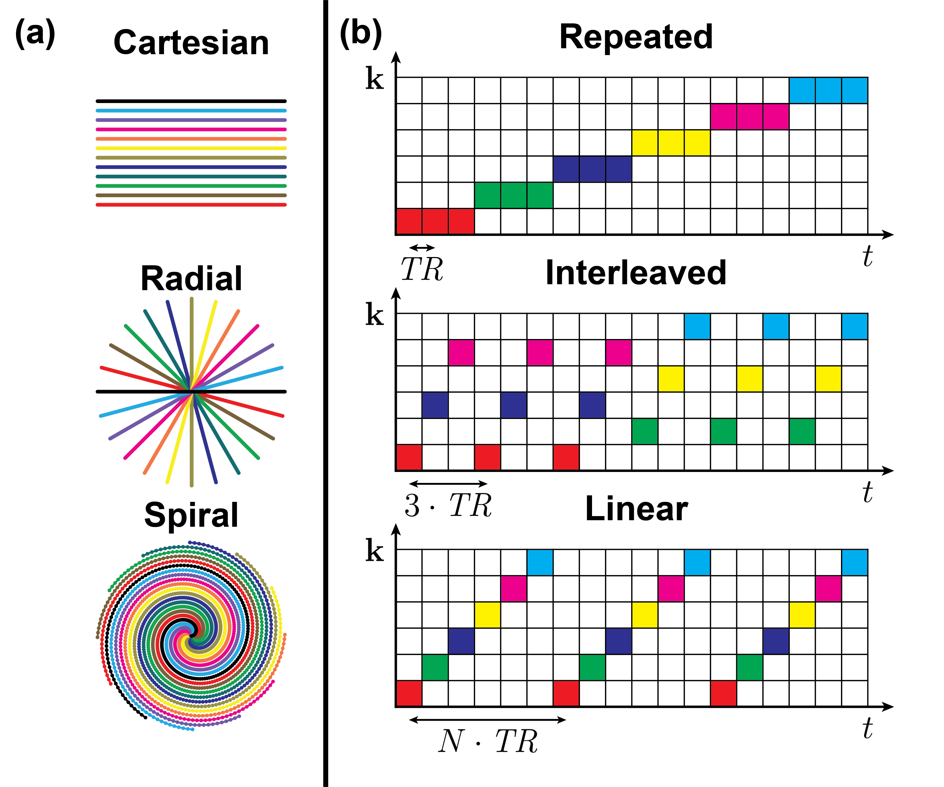
Figure 1: (a) Cartesian (top), radial (middle) and spiral (bottom) sampling trajectories. (b) Schematic representations of the repeated (top), interleaved (middle) and linear (bottom) sampling orderings. Each colored square represents one readout. The repeated ordering samples the same readout multiple times (3 times in this simple schematic, typically dozens of times in practice), while the linear ordering samples all N readouts (12 in our experiments) before repeating. The interleaved ordering is a hybrid between the other two orderings.
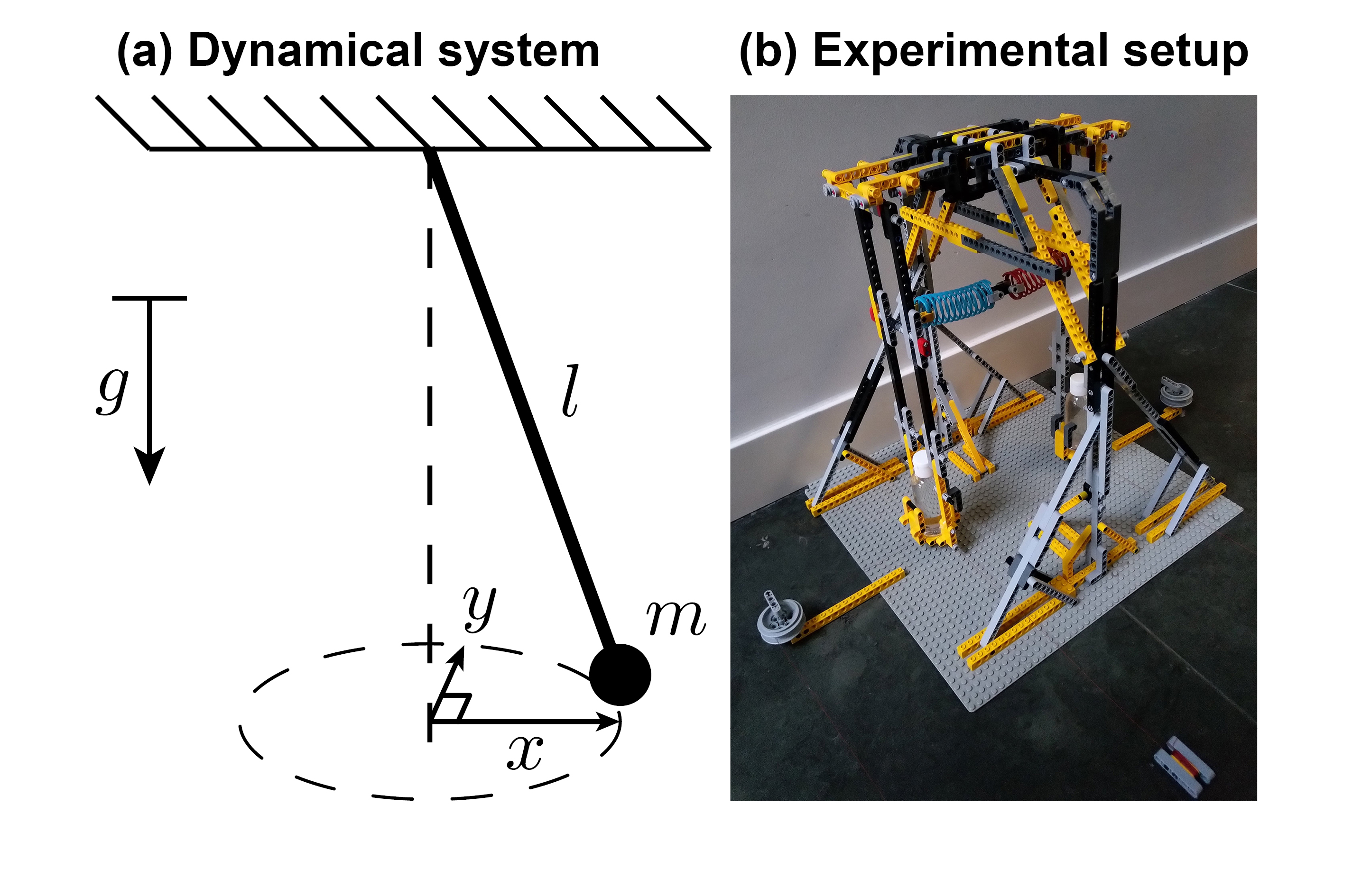
Figure 2: (a) Schematic overview of a spherical pendulum with length $$$l$$$, mass $$$m$$$, and gravitational acceleration $$$g$$$. The pendulum is able to swing in the $$$x$$$- and $$$y$$$-directions, and its tip traces the shape of an ellipse. (b) Experimental setup of the spherical pendulum, with a tube at the end of the pendulum generating MR contrast.
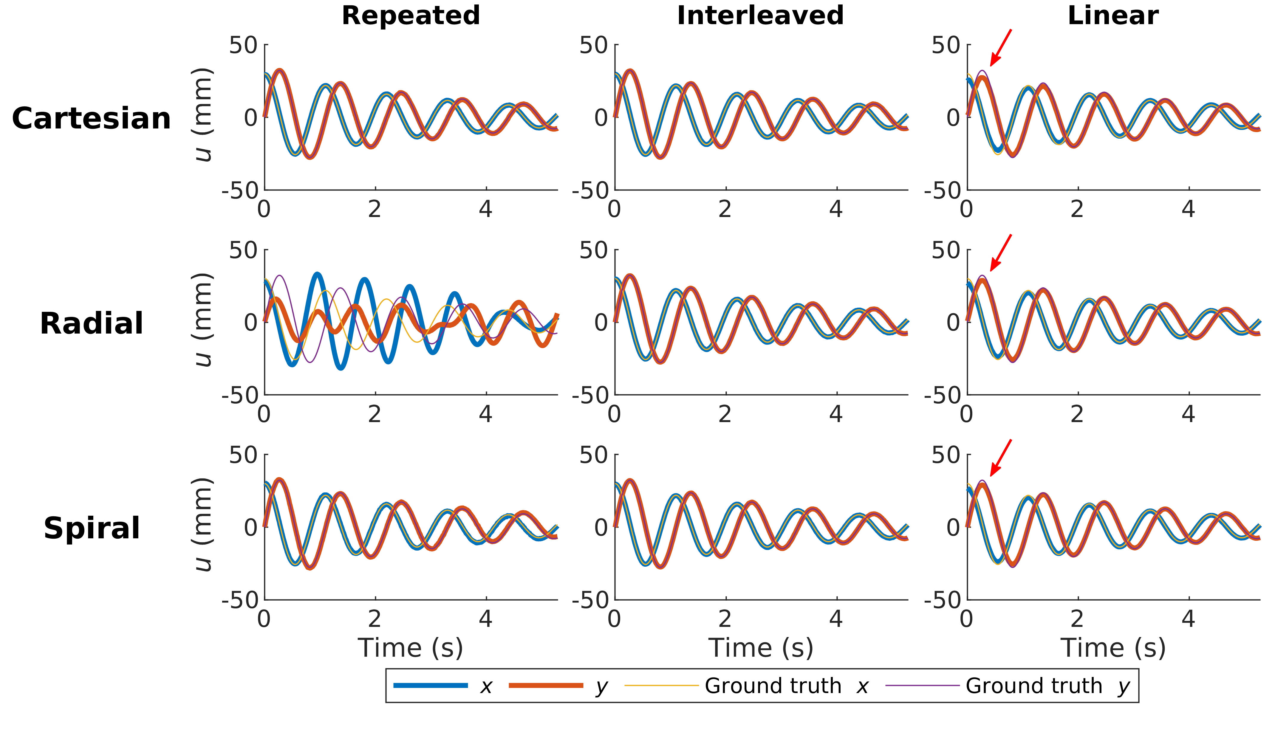
Figure 3: Estimated and ground truth $$$x$$$- and $$$y$$$-displacements for each sampling pattern. The reconstruction for the repeated radial pattern fails since a single radial spoke that crosses the center of k-space does not encode motion perpendicular to the readout direction. The linear ordering has a reduced accuracy for all trajectories (see the errors at the red arrows), as the $$$\Delta{}t$$$ becomes too large for accurate finite differences.
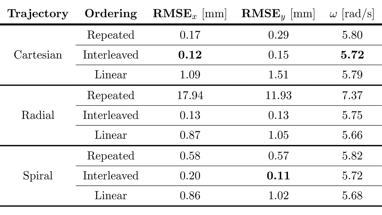
Table 1: RMSE of the estimated displacements in both directions compared to the ground truth, and the estimated frequencies of the dynamical system. The true frequency during simulation was 5.72 rad/s. Bold values indicate the estimations with the smallest error (the estimated frequency for the Cartesian interleaved pattern was slightly more accurate than for the spiral interleaved pattern). The interleaved ordering has the highest accuracy for all trajectories. Also note that the Cartesian trajectory systematically performs worse in the phase encode ($$$y$$$) direction.
Figure 4: (a) Estimated displacements of the spherical pendulum. (b) Reconstructed images at different points in time. The vertical line in (a) indicates the time of the current image. For each time point, all readout lines were corrected to the estimated position as shown in (a), followed by a Fast Fourier transform. The artifacts in the phase encode (vertical) direction are caused by the high undersampling in that direction, while the temporal resolution is equal to the $$$\mathit{TR}$$$ (4.4 ms).