1704
A Fourier representation of the diffusion MRI signal
Chengran Fang1, Demian Wassermann1, and Jing-Rebecca Li1
1INRIA Saclay, PALAISEAU, France
1INRIA Saclay, PALAISEAU, France
Synopsis
The diffusion MRI community lacks a spectral perspective to investigate the intricate relationship between the diffusion MRI signals and cellular structures. Our study proposes a new simulation method that can provide a Fourier representation of the signal. Common spectral methods suffer from the singularity of the heat kernel, which requires infinite Fourier modes. We overcome the singularity by formulating the solution in a convolutional form and splitting the heat kernel into a singular part and a smooth part. Numerical experiments are performed to demonstrate the convergence of our method.
Introduction
Diffusion magnetic resonance imaging is an imaging modality that can probe the tissue microstructure(1-3). However, the relationship between the diffusion MRI signals and cellular structures is still intricate. Numerical simulations can help investigate the relationship, and the Bloch-Torrey equation is the widely accepted theory that models the diffusion MRI signal(4,5). Nevertheless, existing simulation frameworks such as finite element methods cannot provide a Fourier representation of the signal. This study proposes the Fourier Potential Method (FPM) as a new spectral method to solve the Bloch-Torrey equation.The main challenge of spectral methods involves the singularity of the heat kernel. In theory, infinite Fourier modes are required due to the singularity. This limitation may lead to the Gibbs phenomenon that could degrade the approximation accuracy(6).
We formulate the solution of the Bloch-Torrey equation as a convolution with the heat kernel, which is called the single-layer potential. The convolution allows us to split the heat kernel into a singular part and a smooth part to overcome the singularity. We derived an asymptotic formula to approximate the singular part. Moreover, the recursive method proposed by Greengard et al.(7,8) can efficiently evaluate the smooth part. Finally, we numerically validated the convergence of our method and showed the error behavior in several simulation parameters.
Method
We restrict ourselves to the 2D diffusion setting with impermeable interfaces and PGSE diffusion-encoding sequence(9). The main steps of our method are 1) transforming the Bloch-Torrey equation to the diffusion equation using the narrow pulse assumption; 2) formulating the solution of the diffusion equation using the single-layer potential, and splitting it into two parts; 3) approximating the singular part of the single-layer potential using an asymptotic expansion, and storing the smooth part using the Fourier coefficients; 4) computing the diffusion MRI signal using the above representation. We explain each step below. Some mathematical details are omitted due to the length constraint of this abstract.The narrow pulse assumption allows us to transform the Bloch-Torrey equation to a diffusion equation:
\begin{align}\frac{\partial}{\partial t}{w(\textbf{x},t)}&=\nabla\cdot(\mathcal{D}\nabla w(\textbf{x},t)),&\textbf{x}\in\Omega,t\in[0,\Delta-\delta],\\\mathcal{D}\nabla w(\textbf{x},t)\cdot\textbf{n}&=\mathcal{D}N(\textbf{x},t,\textbf{q}),&\textbf{x}\in\Gamma,t\in[0,\Delta-\delta],\\w(\textbf{x},0)&=0,&\textbf{x}\in\Omega,\end{align}where $$$\Omega$$$ represents the diffusion domain whose boundary is $$$\Gamma$$$ and $$$w$$$ describes the magnetization distribution. The vector $$$\textbf{q}$$$ is $$$\frac{\gamma\delta\textbf{g}}{2\pi}$$$ where $$$\textbf{g}$$$ is the magnetic gradient. The Neumann term $$$N$$$ is complex-valued and decays exponentially in time:\begin{equation}N(\textbf{x},t,\textbf{q})= 2\pi\jmath\rho\,\textbf{q}\cdot\textbf{n}e^{-2\pi\jmath\textbf{q}\cdot\textbf{x}}e^{-4\pi^2\mathcal{D}\|\textbf{q}\|^2t},\textbf{x}\in\Gamma,\end{equation}where $$$\rho$$$ is the initial density of the magnetization. According to Haddar et al.(10), the solution of the diffusion equation is:\begin{equation}w(\textbf{x},t)=\int_{0}^{t}\int_{\partial\Omega}\mathcal{D}G(\textbf{x}-\textbf{y},t-\tau)u(\textbf{y},\tau)ds_\textbf{y}d\tau,\textbf{x}\in\Omega,\end{equation}where $$$u$$$ is an unknown function. The heat kernel G is singular when $$$t$$$ is close to 0. To overcome the singularity, we split $$$w$$$ into a singular part and a smooth part. We derived an asymptotic formula for the singular part on the domain boundary $$$\Gamma$$$ and the smooth part has a Fourier decomposition. In short, the two parts are:\begin{equation}w_{singular}(\textbf{x},t)=\int_{t-\eta}^{t}\int_{\partial \Omega}\mathcal{D}G(\textbf{x}-\textbf{y},t-\tau)u(\textbf{y},\tau)ds_\textbf{y}d\tau\simeq\sqrt{\dfrac{\mathcal{D}\eta}{\pi}}u(\textbf{x}, t)+O(\eta^{3/2}),\end{equation}\begin{equation}w_{smooth}(\textbf{x},t)=\int_{0}^{t-\eta}\int_{\partial\Omega}\mathcal{D}G(\textbf{x}-\textbf{y},t-\tau)u(\textbf{y},\tau)ds_\textbf{y}d\tau=\mathcal{D}\sum_{\nu}f(\nu,t)e^{2\pi\jmath\nu\cdot\textbf{x}}.\end{equation}The parameter $$$\eta$$$ is a controlling factor to separate the singular part from the heat kernel $$$G$$$. Finally, the diffusion MRI signal is\begin{equation}s=\mathcal{D}\rho^{-1}\int_{\partial \Omega}\int_{0}^{\Delta-\delta}\overline{N}(\textbf{x},\Delta-\delta-\tau,\textbf{q}) w(\textbf{x},\tau)d\tau ds_{\textbf{x}}+|\Omega|\rho e^{-4\pi^2\mathcal{D}\|\textbf{q}\|^2(\Delta-\delta)},\end{equation}and the magnetization $$$w$$$ is\begin{equation}w(\textbf{x},t)\simeq\mathcal{D}\sum_{\nu=-\nu_{max}}^{\nu_{max}}f(\nu, t)e^{2\pi\jmath\nu\cdot\textbf{x}}\Delta\nu^2+\sqrt{\dfrac{\mathcal{D}\eta}{\pi}}u(\textbf{x},t),\textbf{x}\in\Gamma.\end{equation}The Fourier-type decomposition of the smooth part of diffusion MRI signal appears in the equation above. We use the recursive method proposed by Greengard et al.(7) to efficiently evaluate the unknown function $$$u$$$ and the Fourier coefficients $$$f$$$. To numerically implement this method, we discretize the time domain $$$\left[0,\Delta-\delta\right]$$$ with a time step $$$\Delta t$$$ and the domain boundary $$$\Gamma$$$ is discretized with a spatial step $$$\Delta x$$$. In addition, we truncate the Fourier domain at the frequency $$$\nu_{max}$$$. The spectrum is then discretized with a frequency step $$$\Delta\nu$$$.
Results and Discussion
We validate the convergence of our method for some main discretization parameters. The Matrix Formalism method(11) can compute analytical signals for circles, so we use the Matrix Formalism signals as reference signals $$$s_{ref}$$$. We note the signal simulated by our method as $$$s$$$. We study the relative error, defined by $$$\varepsilon = |s-s_{ref}| /s_{ref}$$$. The geometry on which we conduct the convergence study is a circle of radius $$$r$$$. The default values for the physical parameters are below:- $$$r=\{1,2,4\}\mu m$$$, $$$\mathcal{D}_0=0.002\mu m^{2}/\mu s$$$, $$$u_{\mathbf{g}}=[1,0]^{T}$$$
- $$$\delta=10^{-3}\mu s$$$, $$$\Delta=5,000\mu s$$$, $$$b=\{1,4\}ms/\mu m^{2}$$$
Our method can give a spectral representation for the diffusion MRI signal. To numerically compute the spectrum, we truncate it at $$$\nu_{max}$$$. We present the convergence curves regarding $$$\nu_{max}$$$ in Figure 2. We note that the error decreases exponentially due to the fast decay of Fourier coefficients.
Since our method contains several boundary integrations, we discretize the boundaries by regular polygons. We call the discretized segment length of the boundary $$$\Delta x$$$. Figure 3 illustrates the convergence curves in $$$\Delta x$$$.
Conclusion
This study uses potential theory to derive a Fourier-type representation of the diffusion MRI signal. The splitting of the single-layer potential into two parts avoids the singularity of the heat kernel. It also allows the decomposition of the diffusion MRI signal into the Fourier basis. We numerically validated the convergence of our method and showed the error behavior in several simulation parameters. With proper discretization parameters, the relative error can be less than $$$10^{-4}$$$.Acknowledgements
We want to thank the French National Institute for Research in Computer Science and Automation (Inria) for providing the PhD scholarship of Chengran Fang and all necessary support.References
- Palombo, Marco, Andrada Ianus, Michele Guerreri, Daniel Nunes, Daniel C. Alexander, Noam Shemesh, and Hui Zhang. "SANDI: a compartment-based model for non-invasive apparent soma and neurite imaging by diffusion MRI." NeuroImage 215 (2020): 116835.
- Veraart, Jelle, Daniel Nunes, Umesh Rudrapatna, Els Fieremans, Derek K. Jones, Dmitry S. Novikov, and Noam Shemesh. "Noninvasive quantification of axon radii using diffusion MRI." Elife 9 (2020): e49855.
- Jallais, Maëliss, Pedro LC Rodrigues, Alexandre Gramfort, and Demian Wassermann. "Cytoarchitecture Measurements in Brain Gray Matter using Likelihood-Free Inference." In International Conference on Information Processing in Medical Imaging, pp. 191-202. Springer, Cham, 2021.
- Novikov, Dmitry S., Els Fieremans, Sune N. Jespersen, and Valerij G. Kiselev. "Quantifying brain microstructure with diffusion MRI: Theory and parameter estimation." NMR in Biomedicine 32, no. 4 (2019): e3998.
- Kiselev, Valerij G. "Fundamentals of diffusion MRI physics." NMR in Biomedicine 30, no. 3 (2017): e3602.
- Folland, Gerald B. Fourier analysis and its applications. Vol. 4. American Mathematical Soc., 2009.
- Greengard, Leslie, and John Strain. "A fast algorithm for the evaluation of heat potentials." Communications on Pure and Applied Mathematics 43, no. 8 (1990): 949-963.
- Li, Jing-Rebecca, and Leslie Greengard. "High order accurate methods for the evaluation of layer heat potentials." SIAM Journal on Scientific Computing 31, no. 5 (2009): 3847-3860.
- Stejskal, Edward O., and John E. Tanner. "Spin diffusion measurements: spin echoes in the presence of a time‐dependent field gradient." The journal of chemical physics 42, no. 1 (1965): 288-292.
- Haddar, Houssem, Jing-Rebecca Li, and Simona Schiavi. "Understanding the time-dependent effective diffusion coefficient measured by diffusion MRI: the intracellular case." SIAM Journal on Applied Mathematics 78, no. 2 (2018): 774-800.
- Grebenkov, Denis S. "Laplacian eigenfunctions in NMR. II. Theoretical advances." Concepts in Magnetic Resonance Part A: An Educational Journal 34, no. 5 (2009): 264-296.
Figures
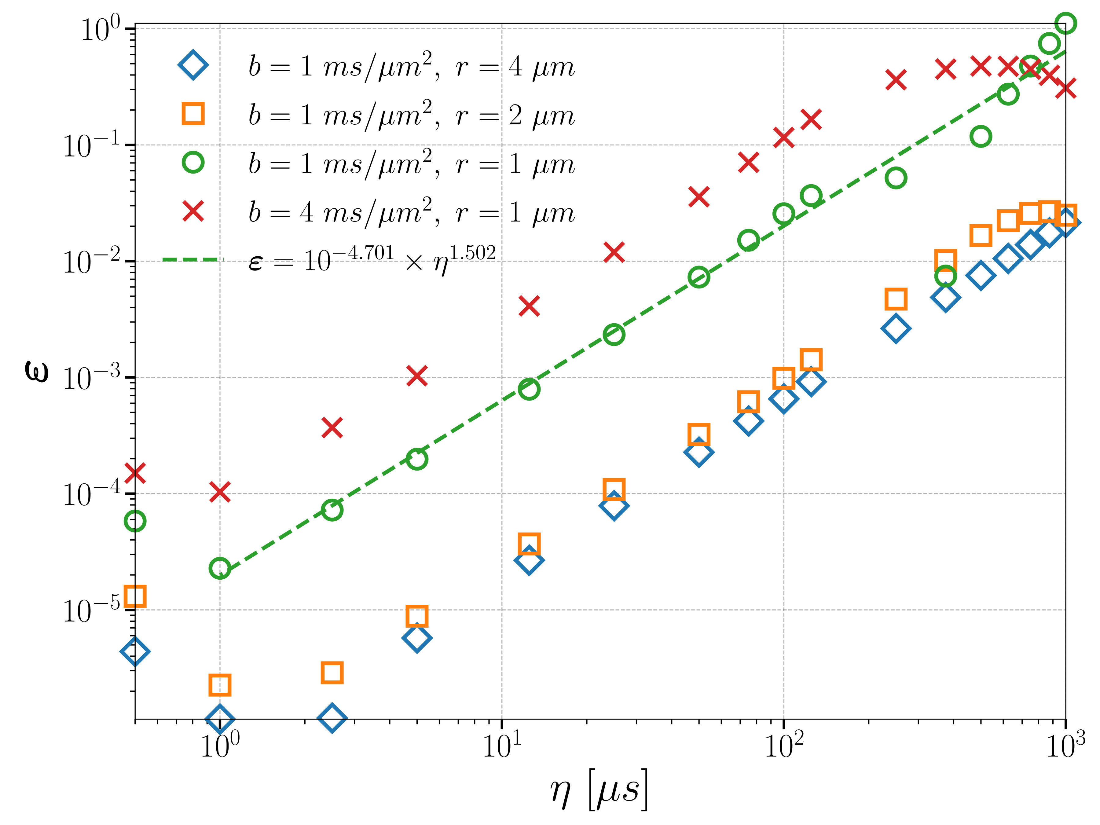
Figure 1: Convergence curves regarding $$$\eta$$$. All other discretization parameters are: $$$\nu_{max} = 10 \mu m^{-1}, \Delta \nu = 0.05 \mu m^{-1}, \Delta x = 0.005 \mu m, \Delta t = 0.5 \mu s$$$. The sampled $$$\eta$$$'s are {0.5, 1, 2.5, 5, 12.5, 25, 50, 75, 100, 125, 250, 375, 500, 625, 750, 875, 1000} $$$\mu s$$$ (from left to right). The slopes of the curves are around $$$3/2$$$.
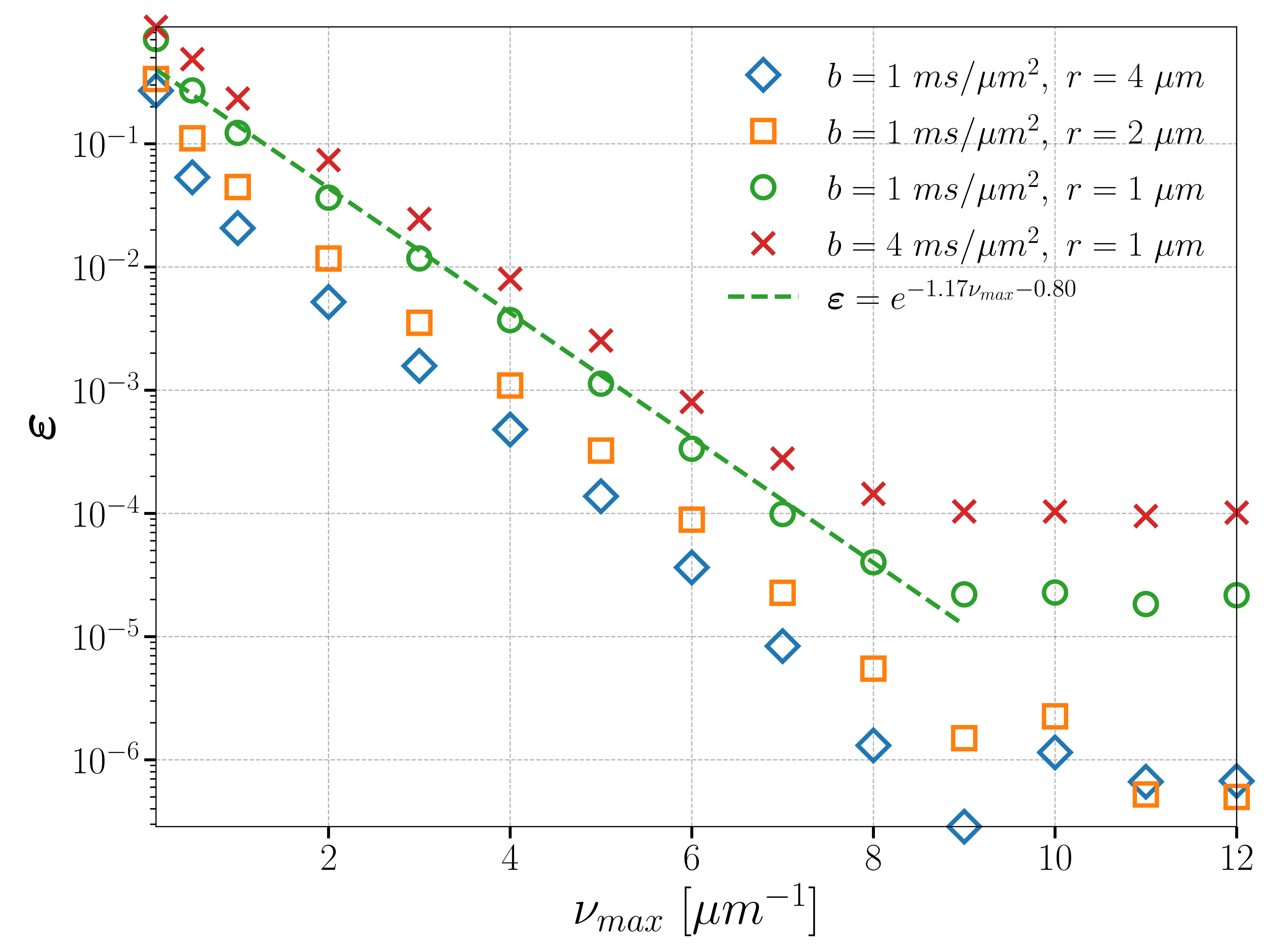
Figure 2: Convergence curves regarding $$$\nu_{max}$$$. All other discretization parameters are: $$$\eta = 1 \mu s, \Delta \nu = 0.05 \mu m^{-1}, \Delta x = 0.005 \mu m, \Delta t = 0.5 \mu s$$$. The sampled $$$\nu_{max}$$$'s are {0.1, 0.5, 1, 2, 3, 4, 5, 6, 7, 8, 9, 10, 11, 12} $$$\mu m^{-1}$$$ (from left to right). We note that the error decreases exponentially due to the fast decay of Fourier coefficients.
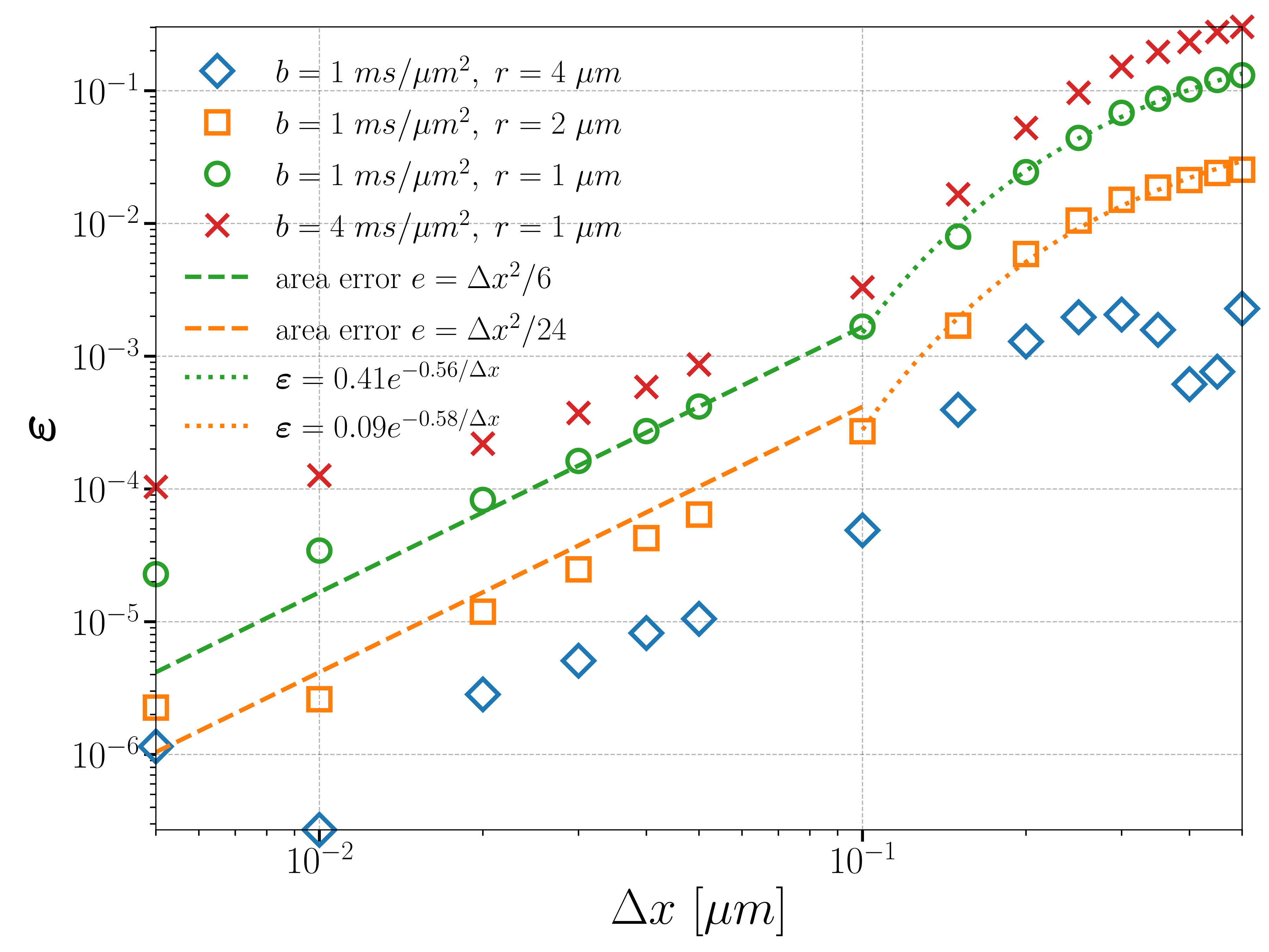
Figure 3: Convergence curves regarding $$$\Delta x$$$. All other parameters are: $$$\eta = 1 \mu s, \nu_{max} = 10 \mu m^{-1}, \Delta \nu = 0.05 \mu m^{-1}, \Delta t = 0.5 \mu s$$$. The sampled $$$\Delta x$$$'s are {0.005, 0.01, 0.05, 0.1, 0.15, 0.2, 0.25, 0.3, 0.35, 0.4, 0.45, 0.5} $$$\mu m$$$ (from left to right). We observe three convergence phases. In the larger range of $$$\Delta x$$$, we observe exponential convergence in $$$1/\Delta x$$$. In the middle range of $$$\Delta x$$$, we observe a convergence of order $$$O(\Delta x^2)$$$. Finally, we observe the curves plateau.
DOI: https://doi.org/10.58530/2022/1704