1643
Orientation dependence of local frequency difference and R2* in parallel versus crossing fibers at 3T and 7T1Department of Radiology and Radiological Sciences, Johns Hopkins University School of Medicine, Baltimore, MD, United States, 2F.M. Kirby Research Center for Functional Brain Imaging, Kennedy Krieger Institute, Baltimore, MD, United States, 3MR Clinical Science, Philips Canada, Mississauga, ON, Canada, 4MRI Clinical Scientist Neuroscience, Philips Healthcare, Best, Netherlands
Synopsis
We investigated the dependence of local frequency difference Δf and R2* on the fiber orientation with respect to the static field in selected parallel-fiber and crossing-fiber regions at 3T and 7T. Δf and R2* showed consistent relationship (sin2θ and sin4θ ) with average ROI-based fiber-to-field angle θ at 3T and 7T. Larger amplitude of variations in Δf and R2* with respect to θ were observed in parallel-fiber compared with crossing-fiber regions indicating non-negligible contributions from fiber orientation dispersion to the nonlinear gradient echo signal evolution and related MRI measures sensitive to white matter microstructure.
Introduction
Previous studies reported the dependence of local frequency difference Δf (from frequency difference mapping, FDM) and R2* on the white matter (WM) fiber-to-field angle θ.1-3 Such orientation dependence and the nonlinear phase evolution of the gradient echo signal have been attributed to the microstructure of the myelin sheath due to its anisotropic magnetic susceptibility1-4. However, whether fiber orientation dispersion, e.g. in crossing fibers, contributes significantly to the Δf and R2* remains unclear. In this study, we investigated the average voxel orientation dependence of Δf and R2* in regions with parallel versus crossing fibers at both 3T and 7T. A single-parameter Δf map was estimated using curve shape parameters derived from a hollow cylinder fiber model (HCFM), while crossing fibers were estimated with multi-shell diffusion MRI.Methods
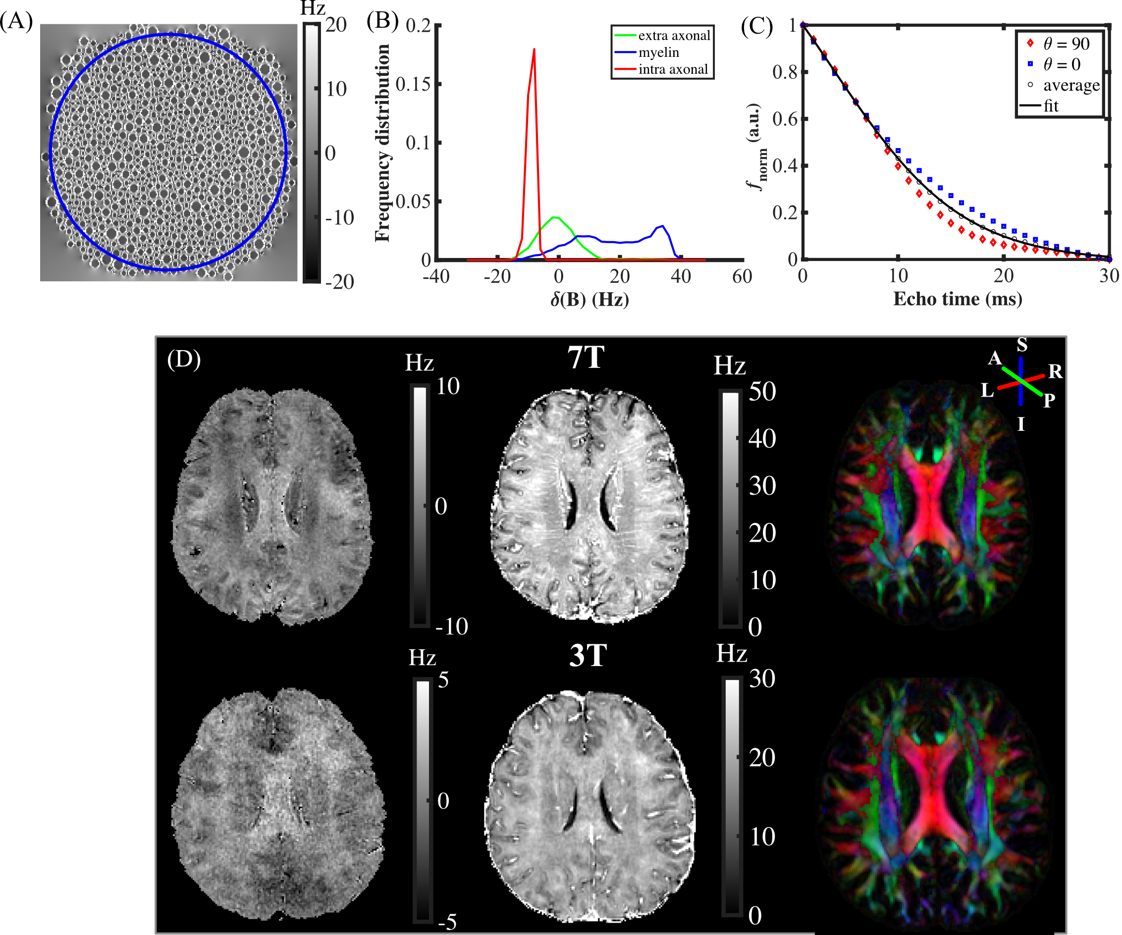
HCFM was used to simulate the field perturbation in WM.1,3 For Δf estimation in vivo, p1 and p2 were calculated using least squares fitting of Eq. (1) to the average of normalized frequency evolution fnorm simulated at θ=0° and θ=90°.$$f=\Delta f\bigl(\frac{exp(-p_1t)}{p_2(exp(-p_1t)-1)+1}\bigr)+C_f\qquad (1)$$
Multi-shell diffusion weighted (DW) EPI MRI scans (voxel size = 1.5×1.5×1.5 mm3, TR = 3350 ms, TE = 86 ms, 7, 46, 46 gradient directions for b = 0, 1500, 3000 s/mm2) were acquired on a 3T Philips scanner. For Δf and R2* measurements, a 3D multi-echo GRE sequence was applied with TR/TE1/∆TE = 44.5/3/3 ms, 12 echoes, voxel size = 1×1×1 mm3 at 3T and TR/TE1/∆TE = 28/5/5 ms, 5 echoes, voxel size = 1×1×1 mm3 at 7T.
The DW images were preprocessed using MRtrix35 and co-registered to GRE space. The θ was determined as the angle between the first peak of the orientation distribution function (ODF) calculated using constrained spherical deconvolution5 and the B0 direction. FDM involved best-path based phase unwrapping6, subtraction of a sixth-order 3D polynomial fit to remove Φ0, subtracting the average frequency across all TE-values and VSHARP7 to get f. The Δf maps were then calculated by least squares fitting of Eq.(1) with fixed p1 and p2 determined from the simulation. R2* maps were reconstructed by mono-exponential fitting to squares of the magnitude data using the power method.8
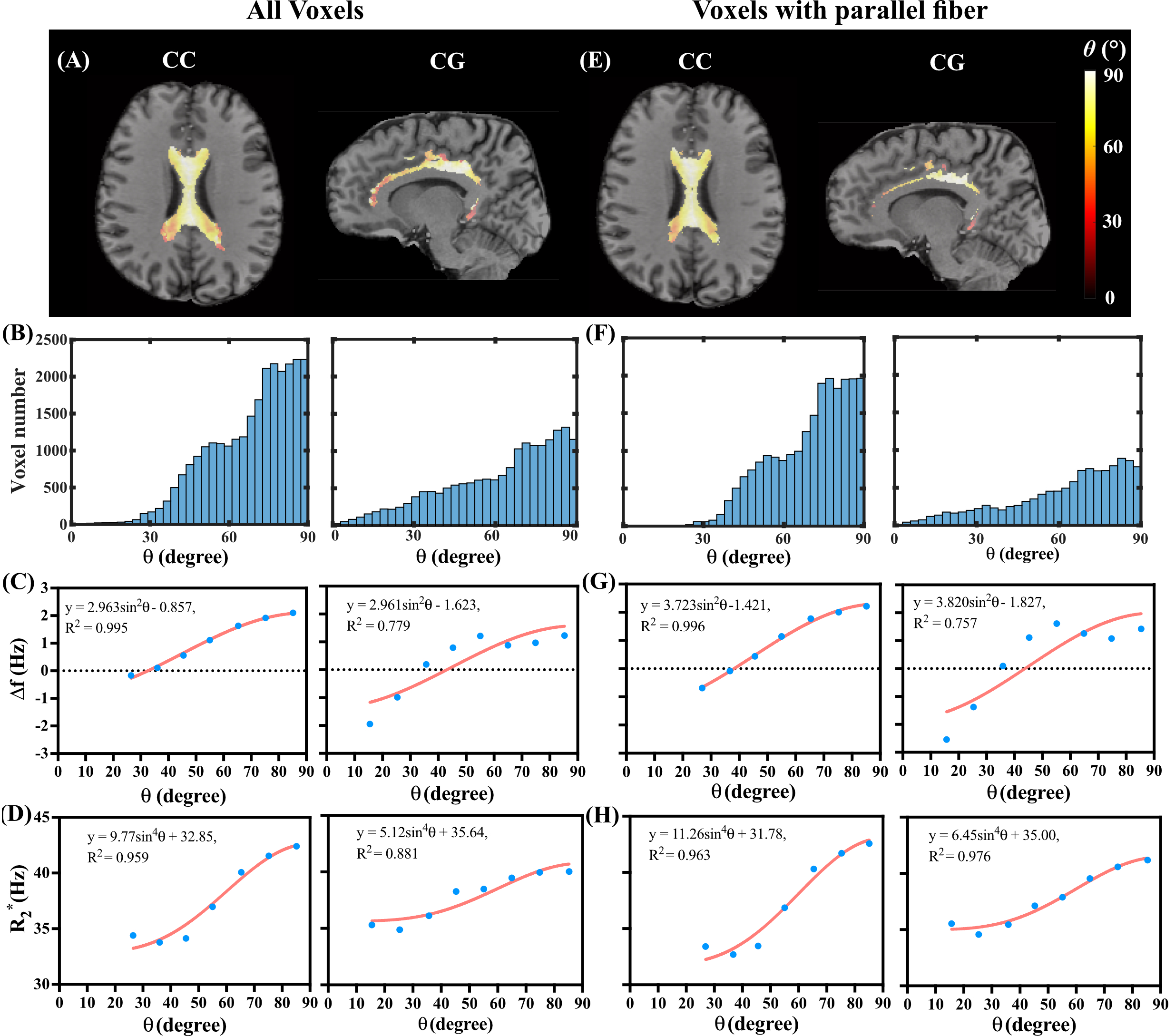
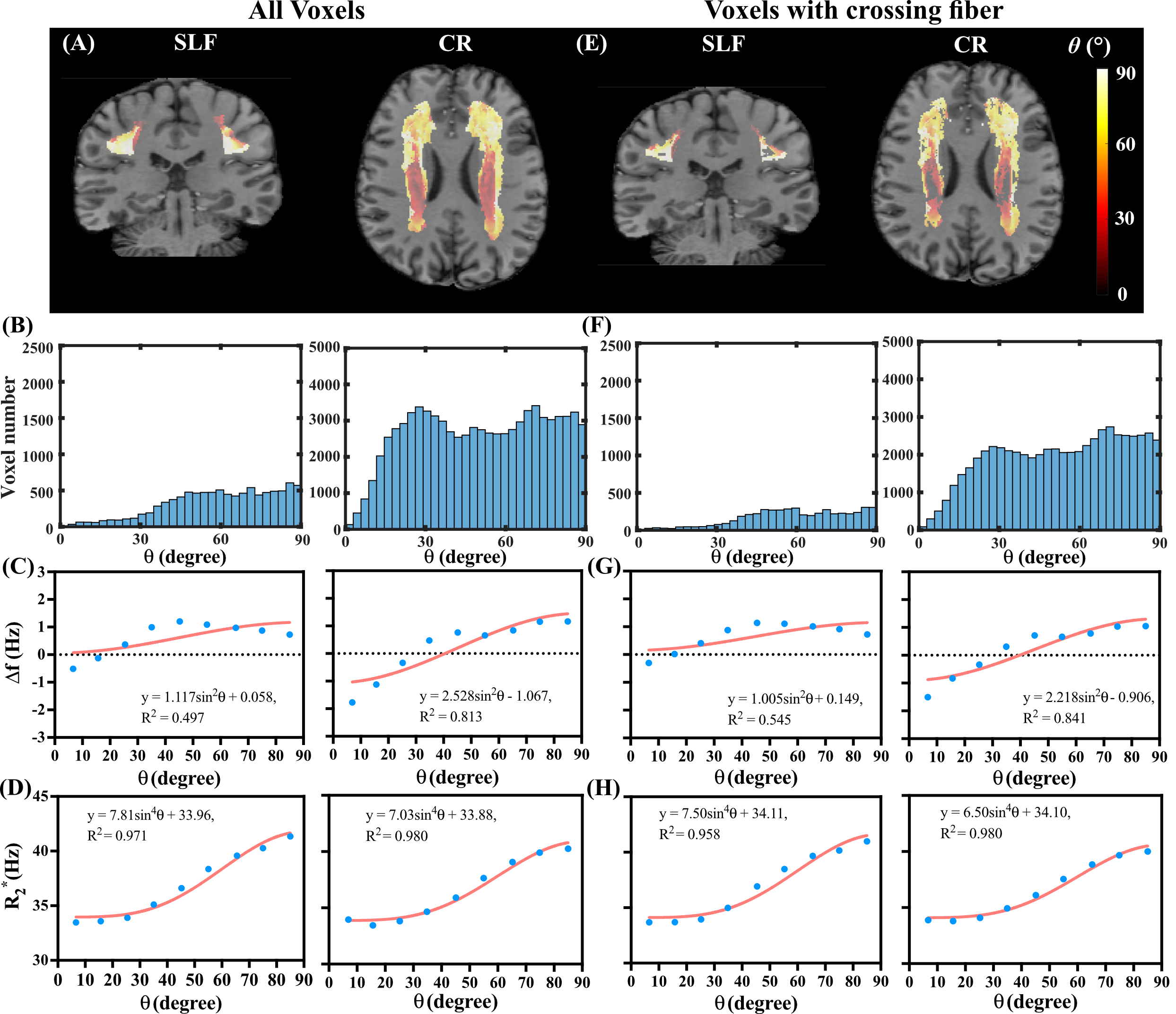
Four ROIs in corpus callosum (CC), cingulum (CG), superior longitudinal fascicles (SLF) and corona radiata (CR) were automatically segmented based on human brain atlases (mricloud.org) using co-registered T1 image for quantifying Δf and R2*. Crossing fiber regions were determined by the voxels where the second peak of ODF was greater than 30% of the first peak. Least squares fitting using sin2θ and sin4θ of the mean θ values in each angular group (9 groups, 10° span for each group) to Δf and R2*, respectively, were performed in both parallel and crossing fiber regions inside each of the four selected ROIs.
Results
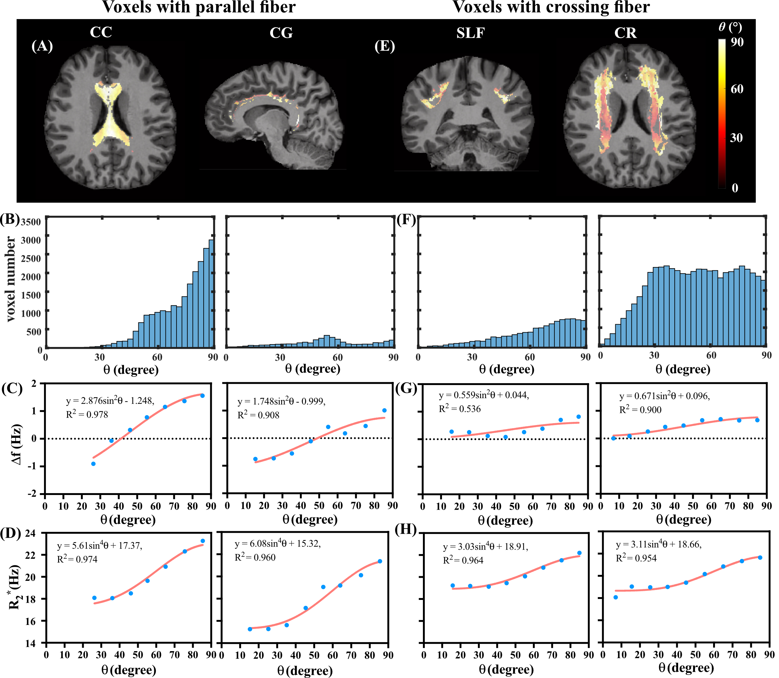
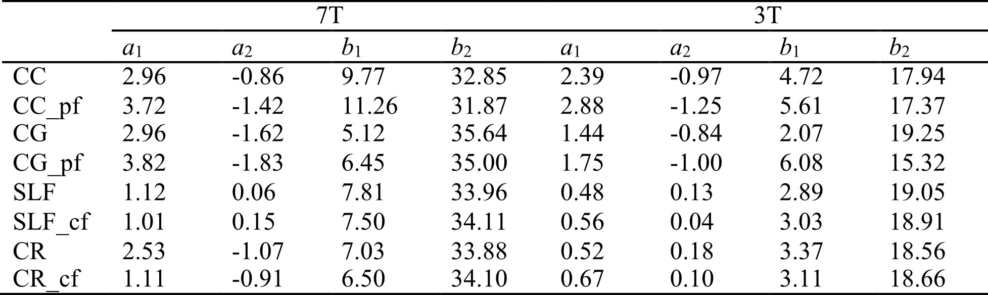
Figure 1(A) and (B) show the simulated field perturbation and frequency distribution for the HCFM with θ=90°. Figure 1(C) shows the variation of normalized frequency over TE curve for θ=0°and θ=90° and the averaged curve with least squares fitting using Eq. (1). The fitting yielded coefficients p1=164s-1and p2=0.66s-1 for 7T and p1=75s-1and p2=0.65s-1 for 3T. Δf maps in vivo calculated by fixed p1 and p2, R2*, and color maps of the first ODF peak are shown in Fig. 1(D). Figures 2(A,B,E,F) show the fiber-to-field angle maps and θ distributions in CC and CG. Most voxels in CC and CG are composed of parallel fibers. The estimated Δf at 7T can be well fitted using Δf=a1sin2θ+a2 (Fig. 2C), with larger coefficients of a1 fitted when excluding crossing fibers in the same bundle (Fig. 2G). Regarding R2*, it exhibits a good fit using R2*=b1sin4θ+b2 (Fig. 2D), with larger b1 and smaller b2 fitted when excluding crossing fiber (Fig. 2H). Figures 3(A,B,E,F) show the fiber-to-field angle maps and θ distributions in SLF and CR. A large portion of voxels in SLF and CR is composed of crossing-fibers. Smaller a1 was fitted when excluding parallel fibers in the same structure (Figs. 3 G versus 3C). Figures 3HvsD show R2* fitted smaller b1 and larger b2 when excluding parallel fibers in SLF and CR (Figs. 3E&F). As illustrated in Figs. 2&3, CC and CG exhibit larger Δf (3-4 Hz) and R2* (6-11 Hz) variations over the relevant θ-range as compared with SLF and CR (1-2.5Hz for Δf and 6-8 Hz for R2*). This can also be seen from the fitted parameters (Table 1). Figures 4 illustrates the θ distributions, orientation dependence of Δf and R2* in four structures acquired at 3T. Despite having the reduced SNR compared to 7T, the measured Δf and R2* showed a consistent pattern of increased orientation dependence with in CC and CG as compared to SLF and CR at 3T.Discussion and conclusion
Using the HCFM, variations in Δf and R2* over the fiber-to-field angle were characterized as Δf=a1sin2θ+a2 and R2*=b1sin4θ+b2 at 3T and 7T. Larger variation amplitudes of Δf and R2* were observed in parallel fiber bundles (CC and CG) as compared to bundles with more crossing fibers (SLF and CR). Further studies with improved biophysical models considering crossing fibers may help better illustrate the relationship of MRI observed Δf and R2* with the underlying tissue microstructures.Acknowledgements
This work was supported by NIBIB (P41EB031771).References
[1] Wharton S, Bowtell R. Fiber orientation-dependent white matter contrast in gradient echo MRI. Proc. Natl. Acad. Sci. U. S. A. 2012;109(45):18559–18564.
[2] Sati P, van Gelderen, Silva AC, et al. Micro-compartment specific T2* relaxation in the brain.Neuroimage, 2013; 77:268-278.
[3] Wharton S, Bowtell R. Gradient echo based fiber orientation mapping using R2* and frequency difference measurements. Neuroimage 2013;83:1011-1023.
[4] Li W, Liu C, Duong T, et al. Susceptibility tensor imaging (STI) of the brain. NMR Biomed, 2017;30(4):e3540.
[5] Tournier, J-D, Calamante F, Alan C. Robust determination of the fiber orientation distribution in diffusion MRI: non-negativity constrained super-resolved spherical deconvolution. Neuroimage 2007;35(4):1459–1472.
[6] Abdul-Rahman HS, Gdeisat MA, Burton DR, et al. Fast and robust three-dimensional best path phase unwrapping algorithm. Appl Opt 2007;46(26):6623-6635.
[7] Schweser F, Deistung A, Lehr BW, et al. Quantitative imaging of intrinsic magnetic tissue properties using MRI signal phase: an approach to in vivo brain iron metabolism? Neuroimage 2011;54(4):2789-2807.
[8] Deistung A, Schafer A, Schweser F, et al. Toward in vivo histology: A comparison of quantitative susceptibility mapping (QSM) with magnitude-, phase-, and R2*-imaging at ultra-high magnetic field strength. Neuroimage 2013;65:299–314.
Figures