1642
How can we reliably mitigate flip angle and fibre orientation dependence in MPM-based R2* estimation at 7T?1Wellcome Centre for Human Neuroimaging, UCL Queen Square Institute of Neurology, University College London, London, United Kingdom, 2Centre de Résonance Magnétique des Systèmes Biologiques, UMR5536, CNRS/University Bordeaux, Bordeaux, France, 3Laboratory for Research in Neuroimaging, Department for Clinical Neuroscience, , Lausanne University Hospital and University of Lausanne, Lausanne, Switzerland, 4Department of Systems Neurosciences, University Medical Center Hamburg-Eppendorf, Hamburg, Germany, 5Department of Neurophysics, Max Planck Institute for Human Cognitive and Brain Sciences, Leipzig, Germany
Synopsis
The apparent transverse relaxation rate ($$$R_{2}^{*}$$$) is influenced by biological features, e.g. iron and myelin content. However confounding factors, such as flip angle (α) and fibre orientation dependence, hinder interpretation. Multi-α data acquired as part of a comprehensive multi-parameter mapping approach can be used to mitigate these confounds. Here we explored how best to do so in vivo at 7T while additionally considering reproducibility. The ESTATICS approach, which assumes a common decay across flip angles, reduced these dependencies. $$$\hat{R_{2}^{*}}$$$, the α-independent component of a heuristic linear model, reduced both dependencies further but was less reproducible than ESTATICS.
Introduction
The apparent transverse relaxation rate ($$$R_{2}^{*}$$$) is influenced by biological features, e.g. iron content1 and myelination2, facilitating in vivo investigation of pathological change3,4. However, confounding factors such as dependence on fibre orientation with respect to B0 (θ)5 and flip angle (α)6 complicate interpretation.The α- and θ-dependence of $$$R_{2}^{*}$$$ stems from the existence of multiple micro-environments within a voxel, e.g. myelin and intra-extracellular compartments, each with distinct relaxation and susceptibility properties. However, it is challenging to quantify these sub-compartments. For robustness, neuroscientific studies commonly make the simplifying assumption of mono-exponential decay obtaining a single $$$R_{2}^{*}$$$ estimate per voxel7.
The time-efficient multi-parameter mapping (MPM) protocol8 acquires multi-echo volumes with two different α to map $$$R_{2}^{*}$$$ as well as the longitudinal relaxation rate (R1) and proton density. Here we explored how these data can be combined to obtain the most α- and θ-robust $$$R_{2}^{*}$$$ estimates. This was assessed at 7T both within and across scanning sessions.
Methods
The effective single compartment $$$R_{2}^{*}$$$ increases linearly with α for a range of residency times and myelin water fractions9. Given multiple α this knowledge can be used to retrieve α-independent ($$$\hat{R_{2}^{*}}$$$) and α-dependent ($$$\frac{dR_{2}^{*}}{d\alpha}$$$ ) components:$$R_{2}^{*}(\alpha)=\hat{R_{2}^{*}}+\frac{dR_{2}^{*}}{d\alpha}\alpha\quad(Eq. 1)$$
In vivo Acquisitions
At 7T, the MPM protocol was extended to acquire four multi-echo (TE=[2.56:2.30:14.5]ms) spoiled gradient echo volumes at nominal α=[6°, 9°, 26°, 42°]. These were chosen to have three pairs suitable for R1 mapping ([6,26]°, [9,26]°, [9 42]°) across which the robustness of different $$$R_{2}^{*}$$$ estimates could be evaluated. TR was 19.5ms, FOV of 192×192×160mm3 with 1mm isotropic resolution. Transmit field inhomogeneity was measured using an in-house sequence exploiting the Bloch-Siegert shift10. The entire imaging session was repeated one week later to assess between-session reproducibility.
Diffusion weighted images with 151 directions and four interleaved b-values of 0, 500, 1000 and 2300s/mm2 were acquired on the same individual at 3T. The ACID toolbox (http://diffusiontools.com/) was used to process the diffusion data and extract θ.
Data Analysis
From the α-pairs (i.e. [6 26]°, [9 42]° and [9 26]°) three $$$R_{2}^{*}$$$ estimates (via log-linear fitting) were obtained:
- $$$R_{2}^{*}$$$ for each α independently
- Applying Eq. 1 to the two per-α estimates to isolate the α-independent component, $$$\hat{R_{2}^{*}}$$$
- Assuming a common decay for each pair using ESTATICS6.
$$COV_{\alpha}=median_{V}\left(\frac{std(\alpha\;datasets)}{mean(\alpha\;datasets)}100\right)\quad(Eq. 2)$$
Reproducibility for each $$$R_{2}^{*}$$$ estimate was assessed over sessions. COVsession was defined as the median, across α-pairs and voxels (V), of the difference between sessions relative to the mean, in percent (Eq.3).
$$COV_{session}=median_{V,\alpha-pairs}\left(\frac{difference\;between\;sessions}{mean\;across\;sessions}100\right)\quad(Eq. 3)$$
The θ-dependence was analysed in WM voxels (probability >0.9, fractional anisotropy >0.6). The voxel-wise fibre orientations with respect to B0, θ(r), were binned and the mean $$$R_{2}^{*}$$$ per bin were plotted against θ(r). The function $$$R_{2}^{*}=R_{2,Iso}^{*}+R_{2,Aniso}^{*}sin^{4}(\theta)$$$, predicted by the hollow cylinder fibre model11, was fit to the data to extract the isotropic component of $$$R_{2}^{*}$$$ ($$$R_{2,Iso}^{*}$$$) and the proportional θ-dependence via $$$R_{2,Aniso}^{*}/R_{2,Iso}^{*}$$$
Results
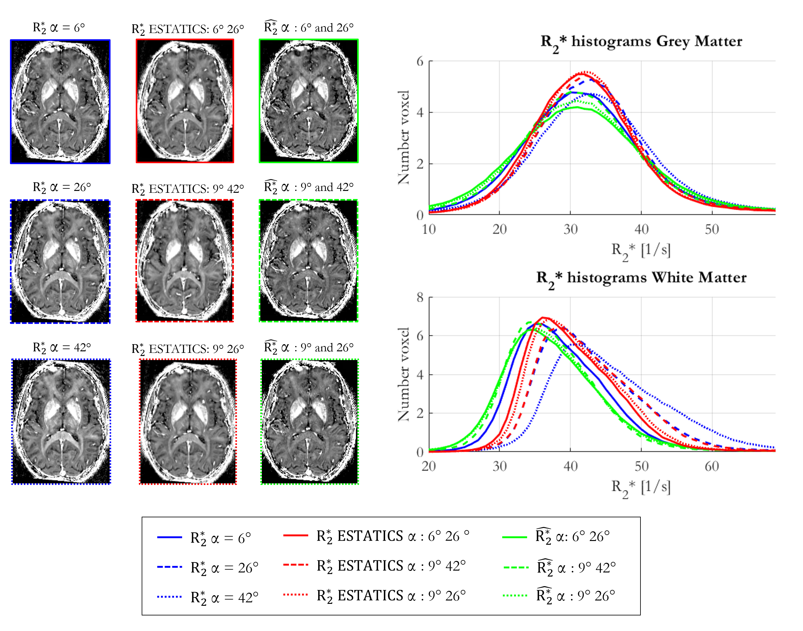
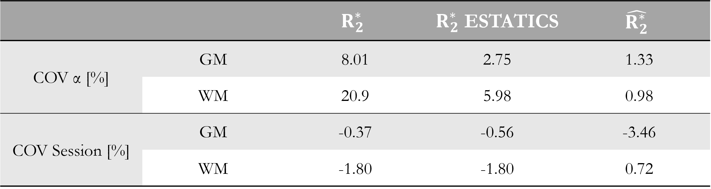
Figure 1 shows $$$R_{2}^{*}$$$ maps from the three approaches. The estimates were comparatively consistent in GM (Figure 1, histograms). However, in WM this was only true of $$$\hat{R_{2}^{*}}$$$. The per-α estimates showed the greatest variability.The repeatability analysis revealed $$$\hat{R_{2}^{*}}$$$ to be most robust to α variation in both GM and WM, while the per-α $$$R_{2}^{*}$$$ estimates were least robust (Table 1).
The reproducibility was highest for $$$\hat{R_{2}^{*}}$$$ in WM (COVsesion=0.72%) but poorest in GM (COVsession=-3.46%). The ESTATICS and per-α $$$R_{2}^{*}$$$ estimates had similar reproducibility in WM (COVsession=-1.80%), which was <1% in GM.
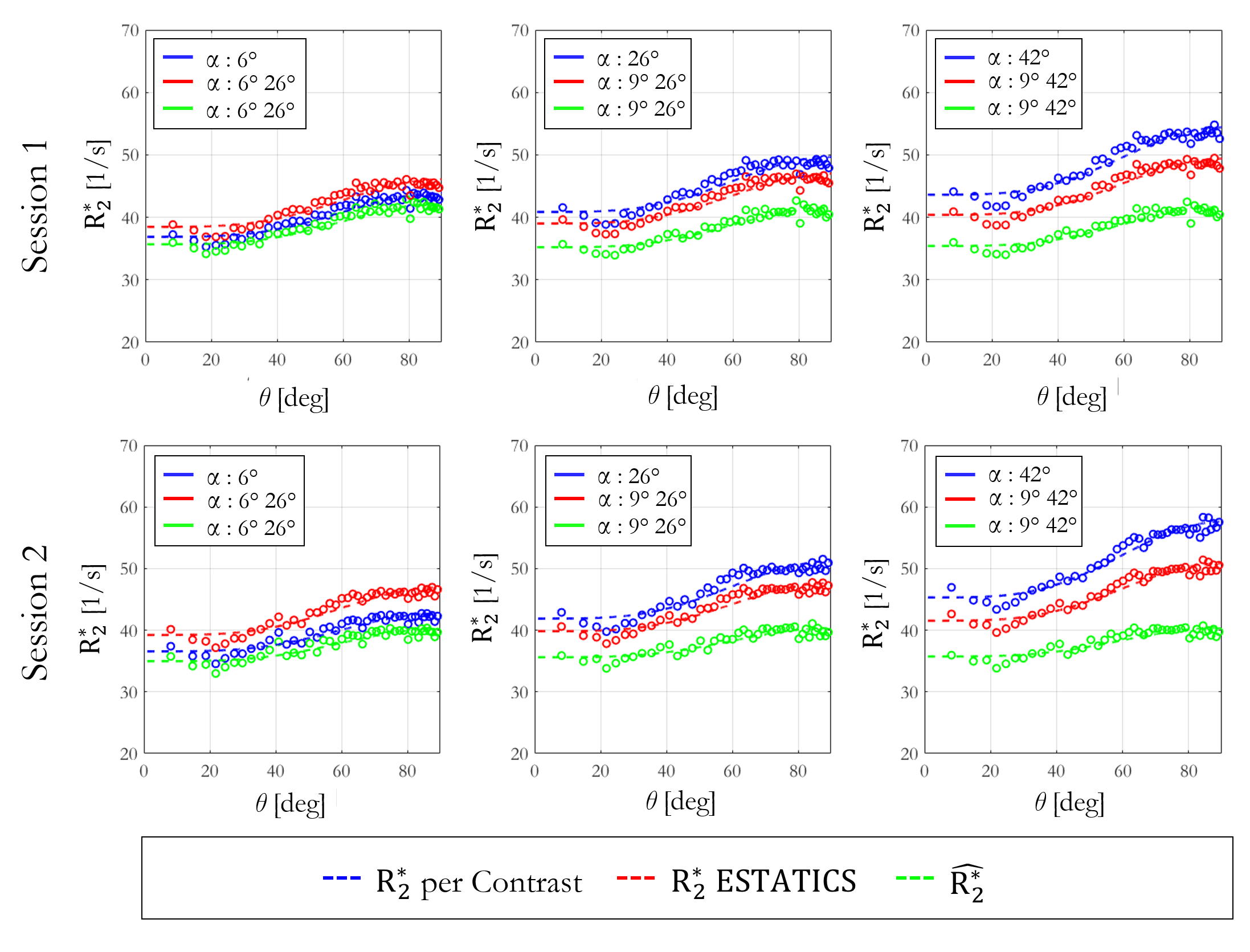
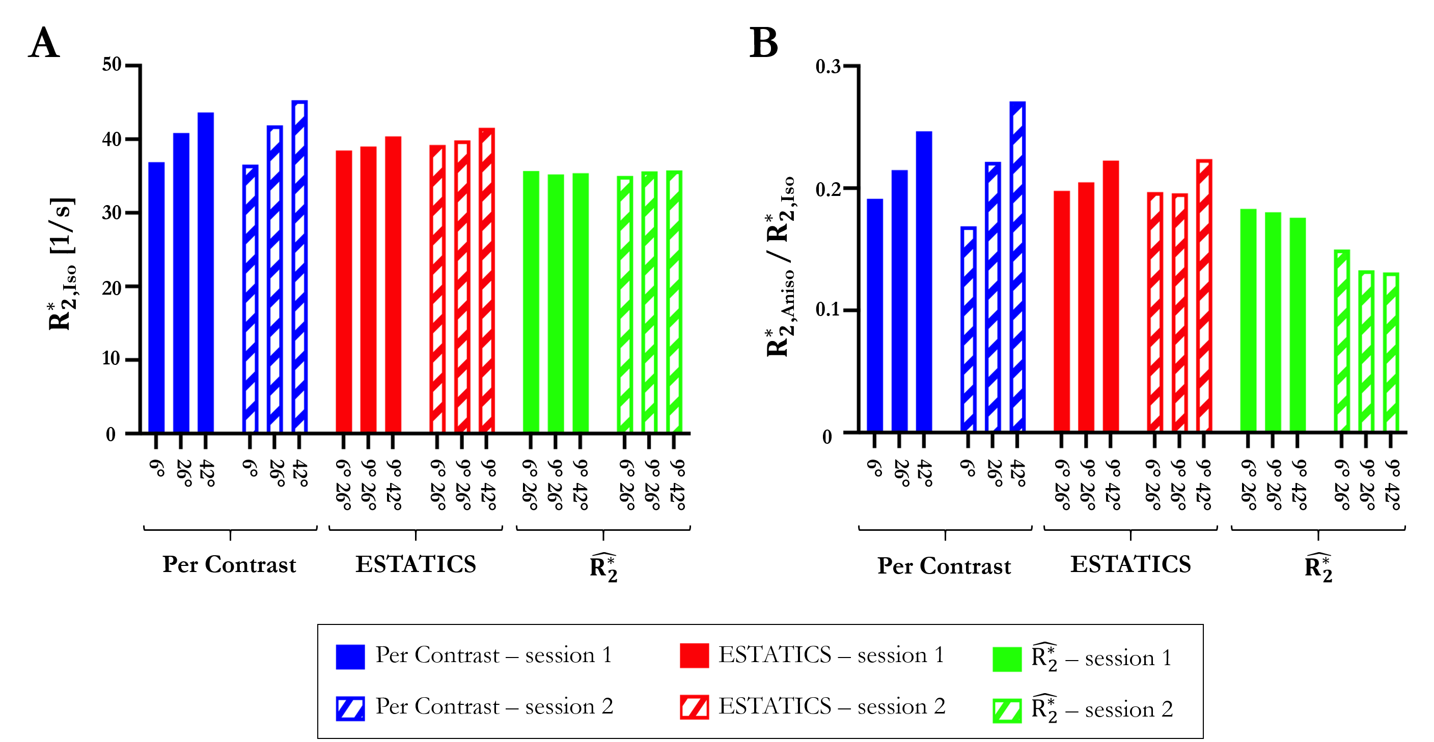
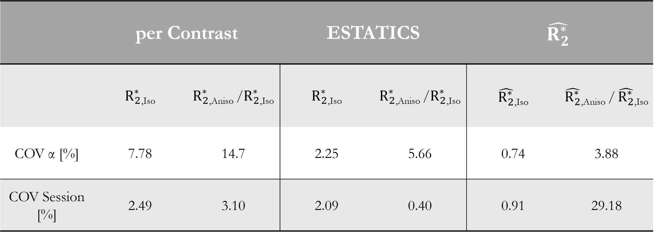
Figure 2 shows the θ-dependence of $$$R_{2}^{*}$$$ estimates across two sessions. $$$\hat{R_{2}^{*}}$$$ provided the most robust quantification of $$$R_{2,Iso}^{*}$$$ (Figure 3A), across both α-pairs and sessions (Table 2, COVα=0.74%, COVsession=0.91%), the least θ-dependence (Figure 3B) and the greatest consistency as α varied (COVα=3.88% versus 5.66% for ETATICS and 14.7% for per-α). However, the anisotropic component derived from $$$\hat{R_{2}^{*}}$$$ had the lowest cross-session reproducibility indicating greater sensitivity to noise (Table 2).
Discussion
We investigated the α- and θ-dependence of $$$R_{2}^{*}$$$ estimates in vivo at 7T, focusing on the mitigation of biases introduced by mono-exponential fitting. $$$\hat{R_{2}^{*}}$$$ was most robust to α variation, particularly in WM and led to a more reproducible $$$R_{2,Iso}^{*}$$$ estimate than the ESTATICS or per-α approaches. $$$R_{2,Iso}^{*}$$$ is of particular interest for biophysical modelling of the gradient echo signal because it can be link to compartmental T2 values and the g-ratio11,12. $$$\hat{R_{2}^{*}}$$$ also depended less on θ regardless of which α-pairs were used. However, low inter-session reproducibility was observed for $$$\hat{R_{2}^{*}}$$$ in GM and for the θ-dependent component ($$$R_{2,Aniso}^{*}$$$), suggesting sensitivity to noise propagation, especially into the $$$R_{2,Aniso}^{*}$$$ component. The ESTATICS approach, default in the hMRI toolbox, is appealing because it exhibited lower α and θ-dependence than the per-α $$$R_{2}^{*}$$$ estimate, with good reproducibility across sessions due to its noise-robust nature.Acknowledgements
The Wellcome Centrefor Human Neuroimaging is supported by core funding from the Wellcome [203147/Z/16/Z].References
1. C. Ghadery et al., “R2* mapping for brain iron: Associations with cognition in normal aging,” Neurobiol. Aging, vol. 36, no. 2, pp. 925–932, 2015, doi: 10.1016/j.neurobiolaging.2014.09.013.
2. F. Bagnato et al., “Untangling the R2* contrast in multiple sclerosis: A combined MRI-histology study at 7.0 Tesla,” PLoS One, vol. 13, no. 3, pp. 1–19, 2018, doi: 10.1371/journal.pone.0193839.
3. Y. Zhao et al., “In vivo detection of microstructural correlates of brain pathology in preclinical and early Alzheimer Disease with magnetic resonance imaging,” Neuroimage, vol. 148, pp. 296–304, 2017, doi: https://doi.org/10.1016/j.neuroimage.2016.12.026.
4. N. Spotorno et al., “Relationship between cortical iron and tau aggregation in Alzheimer’s disease,” Brain, vol. 143, no. 5, pp. 1341–1349, 2020, doi: 10.1093/brain/awaa089.
5. S. Papazoglou et al., “Biophysically motivated efficient estimation of the spatially isotropic R2* component from a single gradient-recalled echo measurement,” Magn. Reson. Med., vol. 82, no. 5, pp. 1804–1811, 2019, doi: 10.1002/mrm.27863.
6. N. Weiskopf, M. F. Callaghan, O. Josephs, A. Lutti, and S. Mohammadi, “Estimating the apparent transverse relaxation time (R2*) from images with different contrasts (ESTATICS) reduces motion artifacts,” Front. Neurosci., vol. 8, no. SEP, pp. 1–10, 2014, doi: 10.3389/fnins.2014.00278.
7. K. Tabelow et al., “hMRI – A toolbox for quantitative MRI in neuroscience and clinical research,” Neuroimage, vol. 194, no. January, pp. 191–210, 2019, doi: 10.1016/j.neuroimage.2019.01.029.
8. N. Weiskopf et al., “Quantitative multi-parameter mapping of R1, PD*, MT, and R2* at 3T: A multi-center validation,” Front. Neurosci., vol. 7, no. 7 JUN, pp. 1–11, 2013, doi: 10.3389/fnins.2013.00095.
9. G. Milotta, C. Nadège, C. Lambert, A. Lutti, S. Mohammadi, and M. F. Callaghan, “Characterisation of the flip angle dependence of R2* in Multi-Parameter Mapping,” 2021.
10. N. Corbin, J. Acosta-Cabronero, S. J. Malik, and M. F. Callaghan, “Robust 3D Bloch-Siegert based B1+ mapping using multi-echo general linear modeling,” Magn. Reson. Med., vol. 82, no. 6, pp. 2003–2015, 2019, doi: 10.1002/mrm.27851.
11. S. Wharton and R. Bowtell, “Fiber orientation-dependent white matter contrast in gradient echo MRI,” Proc. Natl. Acad. Sci. U. S. A., vol. 109, no. 45, pp. 18559–18564, 2012, doi: 10.1073/pnas.1211075109.
12. Wharton S, Bowtell R. Gradient echo based fiber orientation mapping using R2* and frequency difference measurements. Neuroimage. 2013;83:1011-1023. doi:10.1016/j.neuroimage.2013.07.054
Figures