1620

Imaging Off-Center: How far can we move outside the central imaging region

Sebastian Littin¹, Patrick Hucker¹, Maximilian Frederik Russe², Feng Jia¹, Philipp Amrein¹, and Maxim Zaitsev^1,3
¹Department of Radiology, Medical Physics, University Freiburg, Faculty of Medicin, Freiburg, Germany, ²Department of Radiology, University Freiburg, Faculty of Medicin, Freiburg, Germany, ³Center for Medical Physics and Biomedical Engineering, High Field MR Center, Medical University of Vienna, Vienna, Austria

Synopsis

Imaging outside the predefined and optimized FoV may enhance accessibility for interventional MRI procedures. Here we present different measures to assess the encoding capability of gradient systems in off-center regions. Different clinically establishes sequences are compared at 0.55T and 1.5T regarding their imaging capabilities beyond the predefined target regions.

Introduction

MRI systems are usually designed for a spherical or cylindrical target imaging volume. In this wok we want to explore the feasibility of image acquisition beyond the specified and optimized region. Off-center imaging is especially interesting for interventional procedures where accessibility is important. Here we introduce new measures to assess the encoding capability of the gradient system and of the main magnet. Clinically established MRI sequences are compared in off-center image acquisition at an experimental 0.55T MRI and a clinical 1.5T MRI systems.

Methods

For MR imaging three properties are required:

partial orthogonality of three spatial encoding magnetic fields (SEMs) for signal encoding;
a main magnetic field with a reasonable homogeneity for sample magnetization;
sufficiently homogeneous B1 field for excitation.

Non-constant spatial gradients result in image distortions which can be corrected for. Signal encoding for image acquisition requires reasonable gradient strength and orthogonality. Different measures for assessing and optimizing nonlinear gradient coils have been introduced before: These are the local dot-cross product $$(G_x \times G_y \cdot G_z),$$ which represents the locally achievable voxel volume [1] and the the local gradient orthogonality $$(\frac{G_x \times G_y \cdot G_z}{|G_x| \cdot |G_y| \cdot |G_z|})$$ which has been used in [2]. As additional measures to assess imaging capabilities we propose and introduce here the geometric mean gradient $$(\sqrt[3]{|G_x| \cdot |G_y| \cdot |G_z|}))$$ and the gradient anisotropy defined as the difference between the strongest and the weakest gradient normalized to the geometric gradient strength: $$(\frac{max G - minG}{\sqrt[3]{|G_x| \cdot |G_y| \cdot |G_z|}}).$$ An intuitive insight may be gained by looking at the the minimum gradient $$(min(|G_x|, |G_y|, |G_z|))$$ and maximum gradient $$(max(|G_x|, |G_y|, |G_z|)),$$ as well.
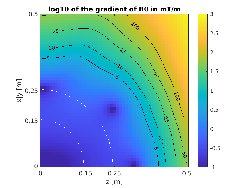
For analyzing the B0 field we chose to look at the gradient of the main field. If the gradient of $$$B_0$$$ is much stronger than the SEMs, imaging is expected to become difficult due to dephasing effects. The resulting deviation of $$$B_0$$$ may prohibit imaging due to bandwidth limits for possible RF-excitations.

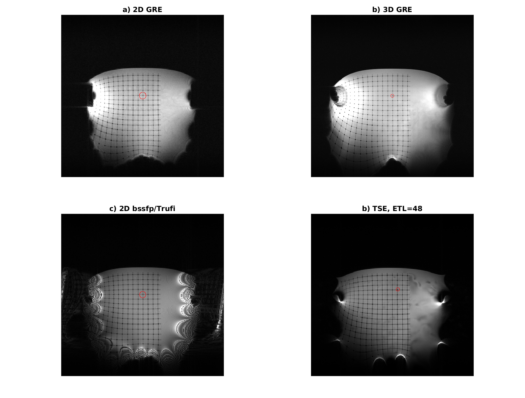
MRI sequences were written in Matlab using the PulSeq [3,4] sequence programming environment. Sequences were optimized to achieve minimum echo time, TE, for the following sequences: 2D gradient echo (2D-GRE) [5], 3D gradient echo (3D-GRE), 2D RARE/TSE [6], 3D RARE/TSE [7], 2D bssfp/Trufi. Imaging experiments were performed on a 1.5T MAGNETOM Aera (Siemens Healthineers, Erlangen, Germany) with XQ Gradients (45 mT/m @ 200 T/m/s) and an experimental 0.55T whole body MRI scanner with an 80cm bore and a gradient system capable of 33 mT/m @ 125 T/m/s. A grid structure with a grid size of 20mm was 3D printed in house to uncover spatial distortions in combination with a large phantom container.

Results

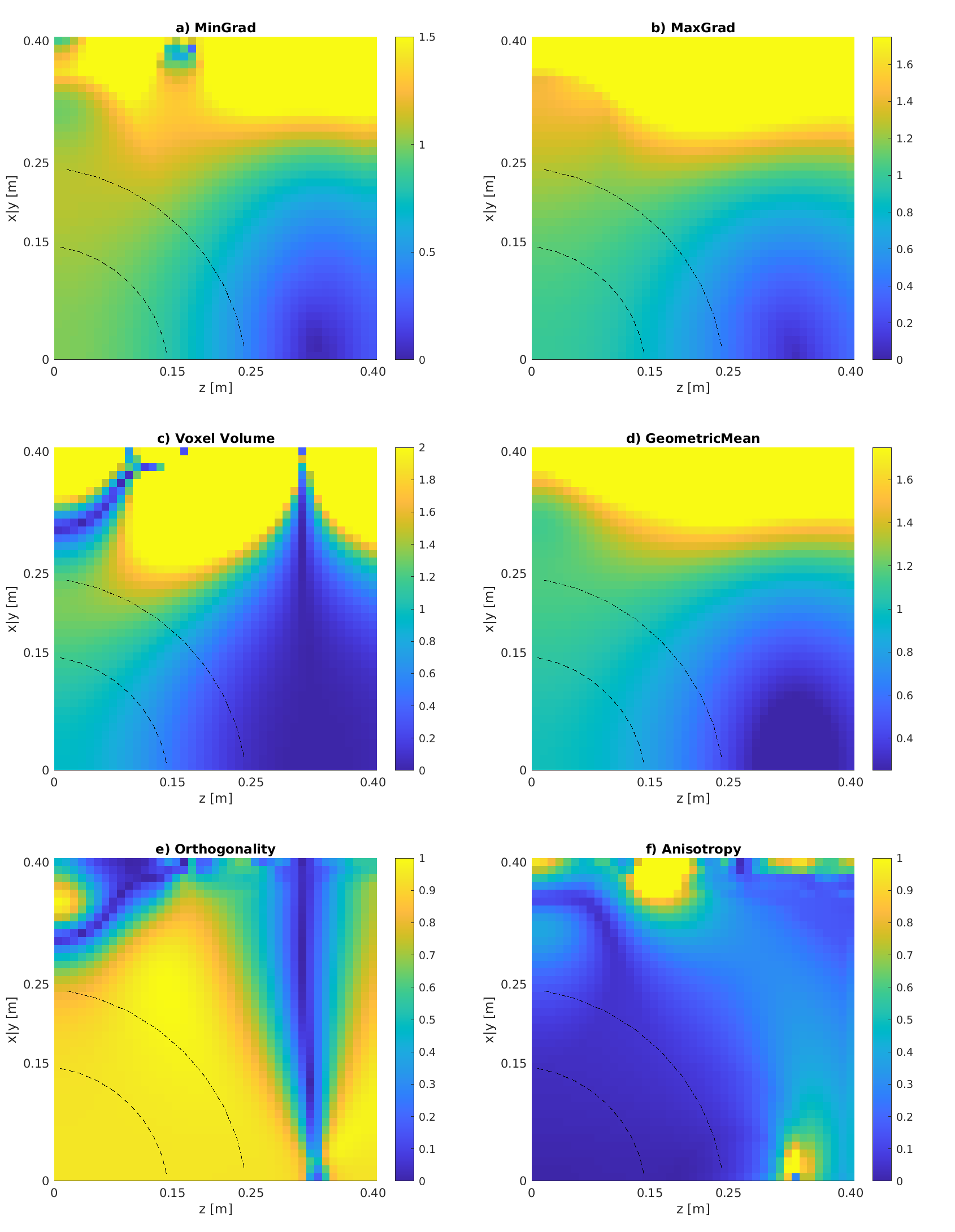
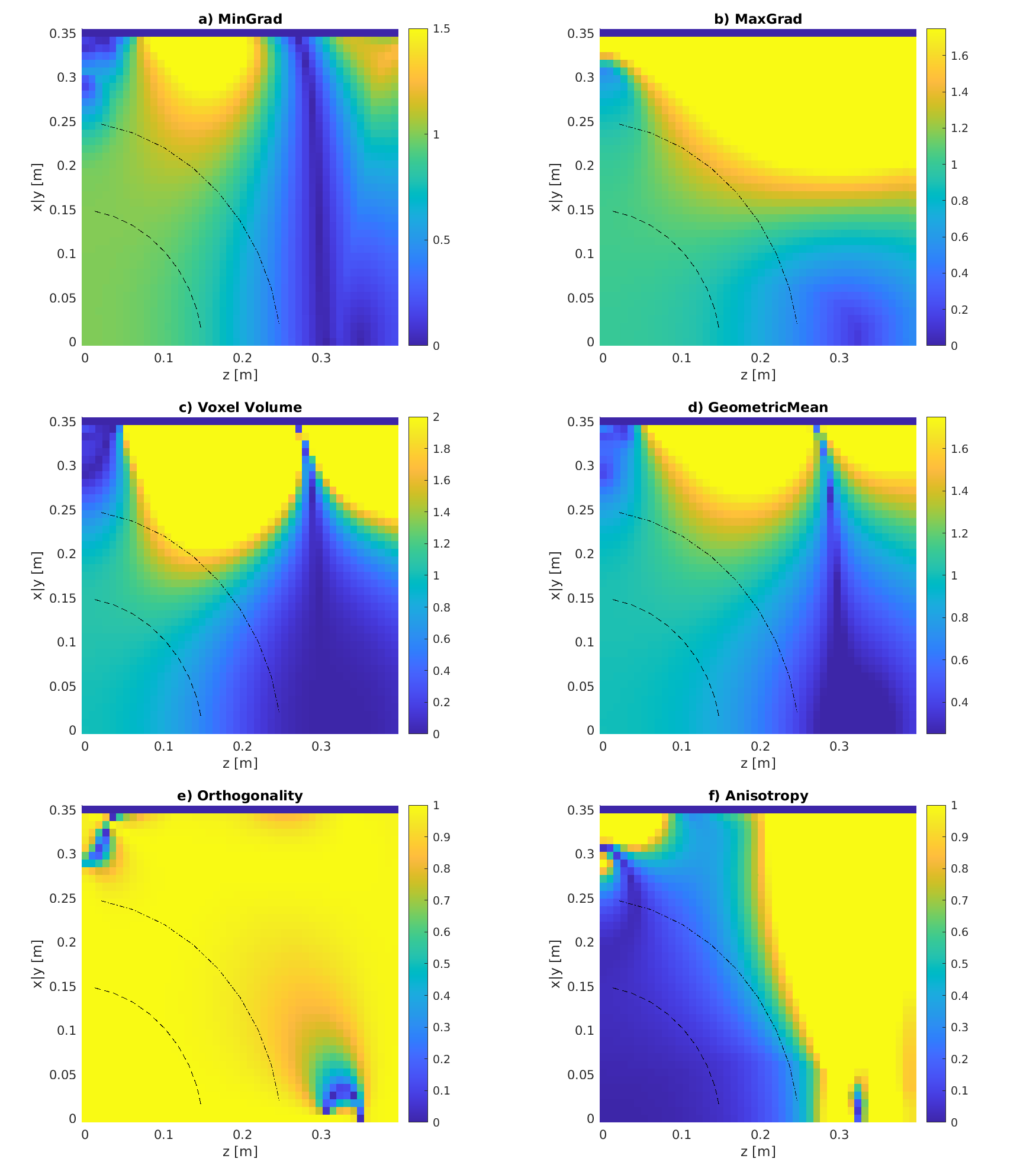
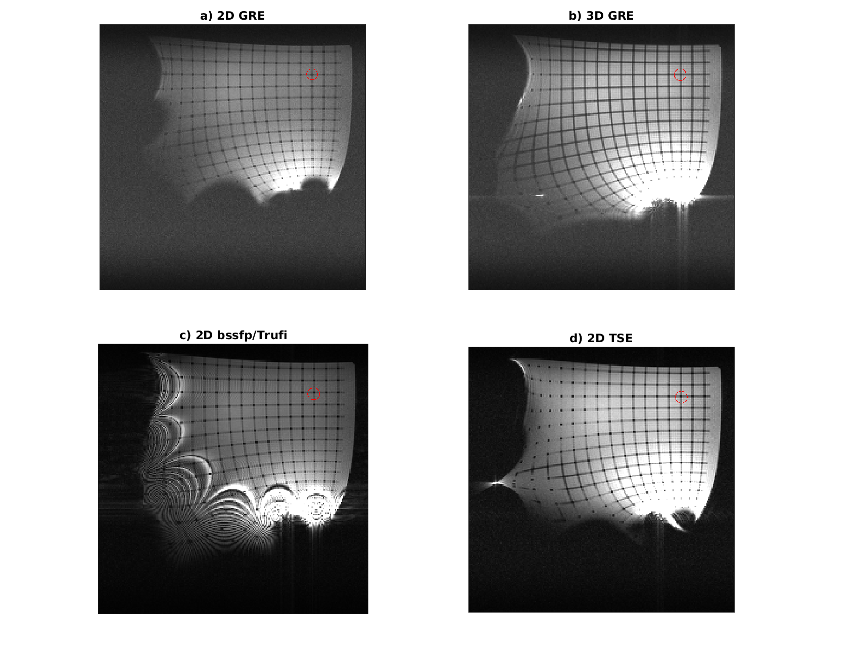
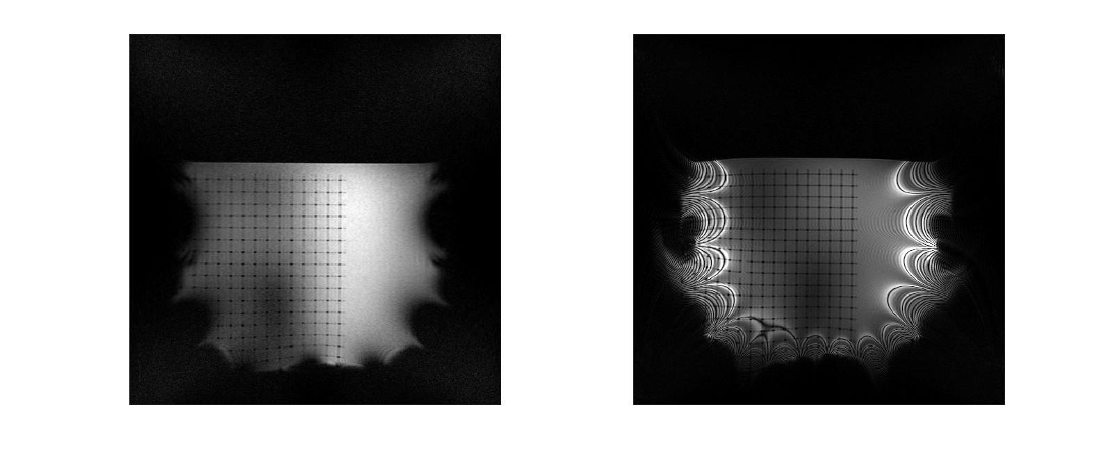
Maps of the different metrics for the encoding fields (dot-cross product, local orthogonality, geometric mean and minimum gradient) are depicted in Fig.1 and Fig.2 for two different gradient systems. A plot of the resulting gradient of the theoretical $$$B_0$$$ field of the 0.55T scanner is shown in Fig.3. Experimental images for different clinically established sequences are depicted in Fig.4 and Fig.5. Distortion corrected images are shown in Fig.6.
In general, 3D sequences seem to be beneficial compared to 2D. Additionally, smaller slice thickness enables for enhanced imaging capabilities off-center which can be explained by through-slice intra-voxel dephasing effects. For TSE acquisitions we found that shorter echo-train-lengths enable for acquiring a larger FoV. The available bandwidth of both systems was not limiting image acquisition.
In comparison the 3D GRE sequence and the bssfp/ TrueFISP (despite severe banding artifacts) sequence reach out the furthest. 0.55T magnets seem to have an enhance region for off-center imaging due to less pronounced gradients of the $$$B_0$$$ field.

Discussion

The feasibility of image acquisition off-center, outside the optimized imaging volume, is limited by the available hardware. It appears that a region moving diagonally out from the iso-center might be especially usefull for image encoding. If this his cone shaped volume is taken into account while designing MRI systems an enhanced imaging volume might become available. The main applications which would benefit from imaging in this region are interventional procedures, eg catheter or needle tracking.
The feasibility of in vivo imaging will be validated in a next step. In addition advanced sequence concepts should be considered, eg missing pulse bssfp [7,8] or others. Larger bore magnets appear to be very promising for extending the FOV. Such magnets may become more widely accessible with the recently established field strength of 0.55T.

Acknowledgements

The authors would like to thank Axel vom Endt and Andrew Dewdney from Siemens Healthineers for supplying the data and for in depth discussions on gradients and shims. Matthias Malzacher, Manuel Schneider, Bernhard Krauss and Martino Leghissa from Siemens Healthineers for support of measurements at the experimental low field system.

The project was funded by the German Federal Ministry of Education and Research under grant number 13GW0356B. The author is responsible for the content of this publication.

References

[1] Littin S, Gallichan D, Welz AM, et al. Monoplanar gradient system for imaging with nonlinear gradients. MAGMA. 2015;28(5):447-457. doi:10.1007/s10334-015-0481-8

[2] Jia F, Schultz G, Testud F, et al. Performance evaluation of matrix gradient coils. MAGMA. 2016;29(1):59-73. doi:10.1007/s10334-015-0519-y

[3] Layton KJ, Kroboth S, Jia F, et al. Pulseq: A rapid and hardware-independent pulse sequence prototyping framework. Magn Reson Med. 2017;77(4):1544-1552. doi:10.1002/mrm.26235

[4] https://pulseq.github.io/

[5] Haase A, Frahm J, Matthaei D, Hänicke W, Merboldt KD. FLASH imaging: rapid NMR imaging using low flip-angle pulses. 1986. J Magn Reson. 2011;213(2):533-541. doi:10.1016/j.jmr.2011.09.021

[6] Hennig, J., Nauerth, A. and Friedburg, H. (1986), RARE imaging: A fast imaging method for clinical MR. Magn Reson Med, 3: 823-833. https://doi.org/10.1002/mrm.1910030602

[7] Patz S, Wong ST, Roos MS. Missing pulse steady-state free precession. Magn Reson Med. 1989;10(2):194-209. doi:10.1002/mrm.1910100205

[8] Kobayashi N, Parkinson B, Idiyatullin D, et al. Development and validation of 3D MP-SSFP to enable MRI in inhomogeneous magnetic fields. Magn Reson Med. 2021;85(2):831-844. doi:10.1002/mrm.28469

Figures

Fig.1: Different measures of the encoding system aka gradients of an experimental 0.55T MRI scanner. Plots are depicted for one quadrant which are due to symmetry reasons a coronal (xz) or saggital (yz) slice orientation. Along the magnet axis (z) the gradients drop rather quickly which is shown by the available minimum (a) and maximum (b) gradient components. The resulting voxels decrease in size (c) moving along the main axis, despite orthogonal SEMs (e). In contrast a higher spatial resolution compared to the main DSV can be expect moving outwards diagonlly.

Fig.2: Measures of the SEMs of an 1.5T MRI scanner. As in the previous example enhanced encoding capabilities may be expected for a region moving diagonally outwards. In this region the minimum gradients increase (a) which results in higher resolution which is represented by the dot-cross product (c) and geometric mean (d). Along the magnet axis the encoding fields drop even more rapid compared to the larger bore previous example. The anisotropy (f) suggest an imaging volume which does not reach much further than the shown DSV of 0.5m along, but allows for encoding in a diagonal region.

Fig.3: Gradients of the main magnetic $$$B_0$$$ field for an experimental 0.55T magnet. Strong field gradients are expected to prohibit imaging due to dephasing effects which cannot be compensated, resulting in signal loss.

Fig.4: Uncorrected images for clinically established sequences 2D gradient echo (a), 3D gradient echo (b), 2D Balanced Steady-State free precession/ TrueFISP (c), 2D Turbo spin echo/ RARE (d). Images were acquired at an experimental 0.55T scanner. Vertical direction in the image corresponds to the z-axis of the scanner (B0 direction). The red circle marks the center of the MR system and imaging volume.

Fig.5: Uncorrected images for clinically established sequences 2D gradient echo (a), 3D gradient echo (b), 2D Balanced Steady-State free precession/ TrueFISP (c), 2D Turbo spin echo/ RARE (d). Images were acquired at an clinical 1.5T scanner. Vertical direction in the image corresponds to the z-axis of the scanner (B0 direction). The red circle marks the center of the MR system and imaging volume.

Fig.6: Corrected images for the 1.5T scanner depict the feasibility of correcting spatial distortions caused by non-constant gradients. Shown are corrected 2D GRE (left) and bssfp (right) images.

Proc. Intl. Soc. Mag. Reson. Med. 30 (2022)

1620

DOI: https://doi.org/10.58530/2022/1620