1611
MORE-SPARKLING: Non-Cartesian trajectories with Minimized Off-Resonance Effects1NeuroSpin, Joliot, CEA, Université Paris-Saclay, F-91191, Gif-sur-Yvette, France, 2Inria, Parietal, Université Paris-Saclay, F-91120, Palaiseau, France, 3Siemens Healthcare SAS, Saint-Denis, 93210, France, 4Siemens Healthineers, Princeton, NJ, United States
Synopsis
We augment the recently introduced SPARKLING algorithm and propose an improved mathematical formulation that takes the temporal dependence of the MR signal into account. This prevents the trajectories from sampling similar portions of k-space at different times, thereby reducing distortions and blurring induced by \(B_0\) inhomogenieties. Overall, these trajectories present a smooth distribution over time in k-space and Minimized Off-Resonance Effects (MORE-SPARKLING), verified both retrospectively and prospectively with scans performed in vivo at 3T on a healthy volunteer.
Introduction
Reducing the scan time in MRI while preserving the highest image quality has been a longstanding goal within the MR community. According to compressed sensing theory, k-space can be optimally undersampled through variable density sampling. Recently, the SPARKLING1 algorithm was introduced to generate sampling patterns that cover the k-space according to a prescribed target sampling distribution (TSD) whereby each k-space trajectory satisfied the MR hardware constraints. This method was successfully extended to 3D2,3, however the presence of amplified patient-induced \(\Delta\text{}B_0\) artifacts was observed3. While the \(B_0\) field inhomogeneities can be addressed through post-processing with correction methods4 without additional scans5, it seems possible to mitigate their impact with improved design of the trajectories.In this work, we incorporate additional components of the MR signal in the formulation of the SPARKLING optimization problem and produce trajectories with Minimized Off-Resonance Effects (MORE) in the final reconstructed MR image.
Theory
Following the original formulation3, a k-space sampling pattern \(\mathbf{K}=(\mathbf{k}_i)_{i=1}^{N_c}\) is composed of \(N_c\) shots, with each 3D shot composed of \(N_s\) samples acquired over the readout duration such that \(\mathbf{k}_i(t)=(k_{i,x}(t),k_{i,y}(t),k_{i,z}(t))\). The trajectory \(\mathbf{K}\) is optimized1,3 as: \[\begin{aligned}\widehat{\mathbf{K}}=\mathop{\mathrm{arg\,min}}_{\mathbf{K}\in\mathcal{Q}^{N_c}}F_p(\mathbf{K})=F_p^{\mathrm{a}}(\mathbf{K})-F_p^{\mathrm{r}}(\mathbf{K})\end{aligned}\] with \(p=N_c\times\text{}N_s\) samplings points, \(\mathcal{Q}^{N_c}\) the \(N_c\)-dimensional set of feasible shots that meet the MR hardware constraints (3), \(F_p^{\mathrm{a}}(\mathbf{K})\) the attraction term which ensures the sampling pattern \(\mathbf{K}\) follows a prescribed TSD \(\rho\) and \(F_p^{\mathrm{r}}(\mathbf{K})\) the repulsion term to avoid clumping of samples. From3, we obtain \(F_p^{\mathrm{r}}(\mathbf{K})\) as: \[\begin{aligned}F_p^{\mathrm{r}}(\mathbf{K})&=\frac{1}{2 p^2}\sum\limits_{1\leq\text{}i,j\text{}\leq p}||\mathbf{K}[i] -\mathbf{K}[j]||_2\end{aligned}\]Ideally, the measured k-space samples \(\mathbf{Y}=(\mathbf{y}_j)_{j=1}^{N_c}\) are given by: \[\begin{aligned}\mathbf{y}_j(t)&=\int\mathbf{x}_{\boldsymbol{r}}\,e^{-(\alpha_{\boldsymbol{r}}+\imath \omega_{\boldsymbol{r}})t}e^{-2\imath\pi(\boldsymbol{\text{k}}_j(t)\cdot\boldsymbol{r})}d\boldsymbol{r}\end{aligned}\] with \(\mathbf{x_r}\) the transverse magnetization of the object, \(\alpha_{\boldsymbol{r}}\) the \(T_2^*\) decay and \(\omega_{\boldsymbol{r}}\) the off-resonance at voxel \(\boldsymbol{r}\). Note the temporal dependence of \(\mathbf{Y}\) on \(\alpha_{\boldsymbol{r}}\) and \(\omega_{\boldsymbol{r}}\), not considered in the original SPARKLING formulation. This results in trajectories that may be locally inconsistent because close samples may be collected at different times (Fig.1(A)), leading to amplified \(\Delta\text{}B_0\) artifacts as observed in3.
Methods
We propose to mitigate the impact of \(B_0\) inhomogeneities by adding the following temporal weights in the repulsion term \(F_p^{\mathrm{r}}(\mathbf{K})\) as: \[\begin{aligned}F_p^{\mathrm{r}}(\mathbf{K})=\frac{1}{2 p^2}\sum\limits_{1\leq\text{}i,j\text{}\leq\text{}p} e^{|t_i-t_j|} ||\mathbf{K}[i]-\mathbf{K}[j]||_2\end{aligned}\] where \(t_i\) and \(t_j\) correspond to the times when the samples \(\mathbf{K}[i]\) and \(\mathbf{K}[j]\) are acquired. Note that \(e^{|t_i-t_j|} \geq 1\), thereby increasing the repulsion term between temporally spaced out points. While generating the modified trajectories, large k-space holes are observed in Fig.1(B) as increased repulsion occurs in regions where the trajectories that start and end nearly at the same location along a plane. To address this issue, we benefited from the multi-resolution sampling design implemented in SPARKLING3 which starts by spreading \(p_{i_{\mathrm{max}}}=p/2^{i_{\mathrm{max}}}\) samples at the maximal \(i_{\mathrm{max}}=5\) decimation levels and iterates through a dyadic process, i.e. \(p_{i_{\mathrm{max}}-i}=2^i p_{i_{\mathrm{max}}}\) for \(i=1:5~(p_0=p)\). Here, we introduce the temporal weighting in the optimization process, and we call \(TW_i,~i=0:2\), when this weighting is activated up to to the decimation step \(i\) with \(p_{i_{\mathrm{max}}-i}\) samples. This results in significantly reduced k-space holes for \(TW_1\) and \(TW_2\) as presented in Fig.1(C)-(D).To evaluate this advancement, different \(T_2^*\) volumes were acquired on a phantom and a healthy volunteer at 3T using a 64-channel head/neck coil array, paired with additional \(\Delta\text{}B_0\) field maps. All acquisitions parameters are detailed in Fig.[fig:acquisitions]. For in vivo scans, a Cartesian GRAPPA4-accelerated reference was also acquired to perform a retrospective study, by simulating the \(B_0\) inhomogeneities4 using the acquired field map (Fig.3). On the phantom, volumes were collected in standard conditions with low artifacts (Fig.4(1)), then \(B_0\) inhomogeneities were added by degrading the machine \(B_0\) shimming (Fig.4(2)).
All image reconstructions were performed using the self-calibrated approach6 and implemented in pysap-mri7.
Results
The retrospective study on a volunteer (Fig.3) shows a quality peak for \(TW_1\) with an improved PSNR by 3dB compared to the original SPARKLING. Aside from sensitivity and registration differences, the retrospective study shows realistic \(B_0\) inhomogeneity simulation compared to prospective in vivo acquisitions (Fig.5). While \(TW_1\) brings better k-space coverage than \(TW_0\), as visible in Fig.1 (B1, C1), \(TW_2\) mostly shows a less mitigated impact of \(\Delta B_0\) artifacts (red/yellow arrows).The prospective study on the phantom (Fig.4) shows significant improvements over \(B_0\) inhomogeneities with temporal weights (blue arrows), decreasing with \(TW_1\) and \(TW_2\) (red arrows). However, without inhomogeneities \(TW_0\) shows slightly degraded quality (B1, yellow arrows) over other trajectories. Similar results are observed in vivo (Fig.5) with more signal for MORE-SPARKLING in \(\Delta\text{}B_0\) regions (blue arrows). Importantly, sharper details and a cleaner contrast are recovered using \(TW_1\) (E, red/yellow arrows). Overall, \(TW_1\) shows improvements over \(TW_0\) that can be attributed to balanced repulsion and reduced k-space holes.
Conclusion
In this work, we present a significant advancement to the SPARKLING formulation which takes the temporal nature of the signal acquisition into account, resulting in MORE-SPARKLING trajectories that exhibit reduced \(\Delta\text{}B_0\) artifacts.However, our first proposition to tackle this problem resulted in the apparition of k-space holes during the optimization process due to increased repulsion. Although we addressed this issue by disabling the temporal weighting prior to the final decimation step, more generic solutions could be achieved by further improving further the formulation. These aspects will be addressed in future works.
Acknowledgements
The concepts and information presented in this article are based on research results that are not commercially available. Future availability cannot be guaranteed. This work was granted access to the HPC resources of IDRIS under the allocation 2021-AD011011153 made by GENCI. Chaithya G R was supported by the CEA NUMERICS program, which has received funding from the European Union’s Horizon 2020 research and innovation program under the Marie Sklodowska-Curie grant agreement No 800945.References
1. Lazarus, C., and others (2019). SPARKLING: variable-density k-space filling curves for accelerated T2*-weighted MRI. mrm 81, 3643–3661.
2. Lazarus, C., and others (2020). 3D variable-density SPARKLING trajectories for high-resolution T2*-weighted magnetic resonance imaging. nmrb.
3. Chaithya, G.R., and others (2021). Optimizing full 3D SPARKLING trajectories for high-resolution T2*-weighted Magnetic Resonance imaging.
4. Fessler, J.A., Lee, S., Olafsson, V.T., Shi, H.R., and Noll, D.C. (2005). Toeplitz-based iterative image reconstruction for mri with correction for magnetic field inhomogeneity. IEEE Transactions on Signal Processing 53, 3393–3402.
5. Daval-Frérot, G., and others (2021). Off-resonance correction for non-Cartesian SWI using internal field map estimation. In 29th proceedings of the ismrm society.
6. El Gueddari, L., Lazarus, C., Carrié, H., Vignaud, A., and Ciuciu, P. (2018). Self-calibrating nonlinear reconstruction algorithms for variable density sampling and parallel reception mri. In 2018 ieee 10th sensor array and multichannel signal processing workshop (sam) (IEEE), pp. 415–419.
7. Gueddari, L.E., and others (2020). PySAP-MRI: a Python Package for MR Image Reconstruction. In ISMRM WS on Data Sampling and Image Reconstruction.
Figures
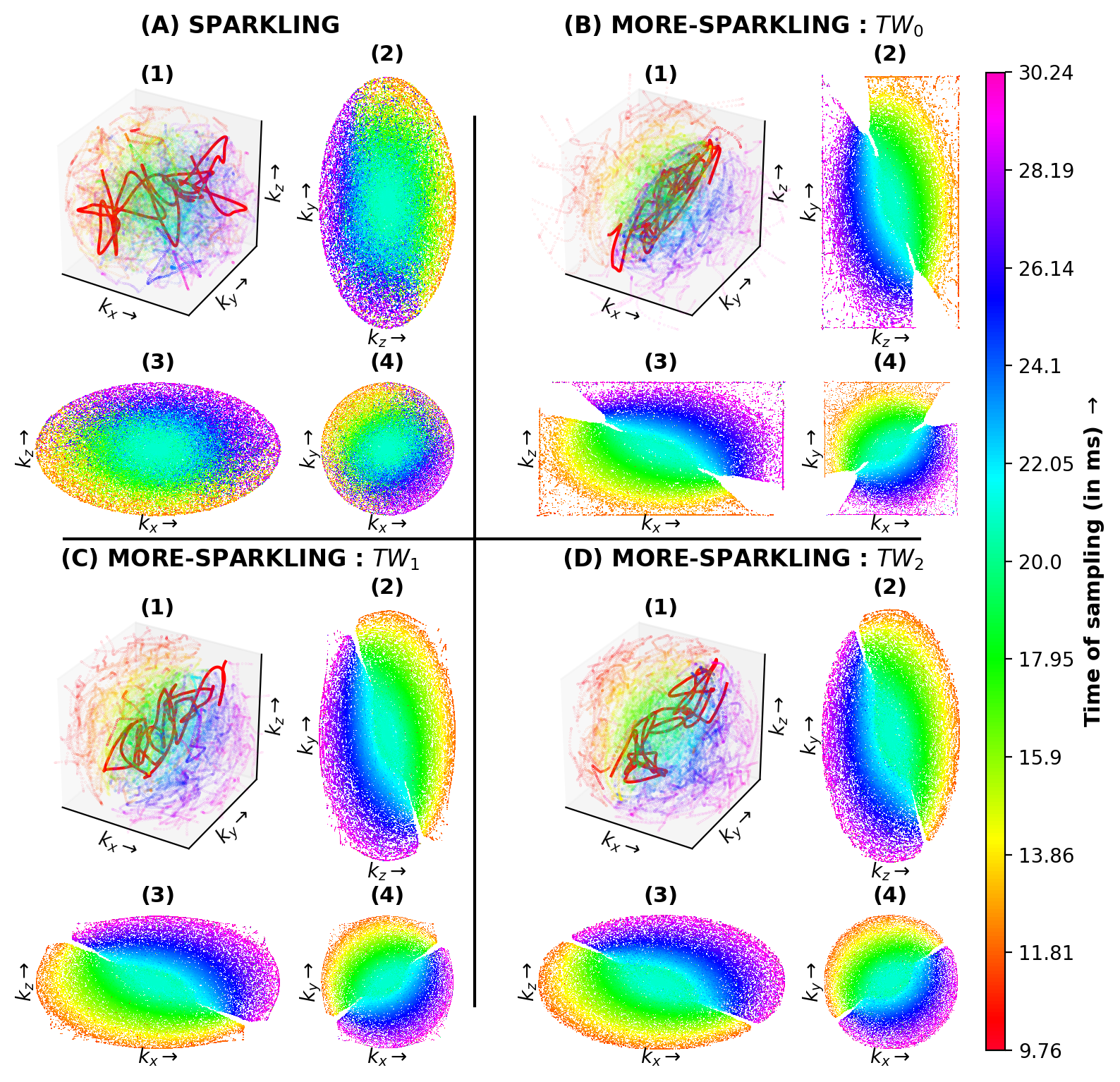
Comparison of different SPARKLING trajectories generated with \(N_c=5329\) (AF=15), \(N_s=2048\) : (A) Without temporal weights, (B) with \(TW_0\), (C) with \(TW_1\), and (D) with \(TW_2\). In each case, the 3D sampling pattern is shown in (1) and the mid-plane k-space slices along (2) \(k_x\)-axis, (3) \(k_y\)-axis and (4) \(k_z\)-axis. A rainbow coloring scheme overlays the sampling trajectories to encode the time in k-space samples.

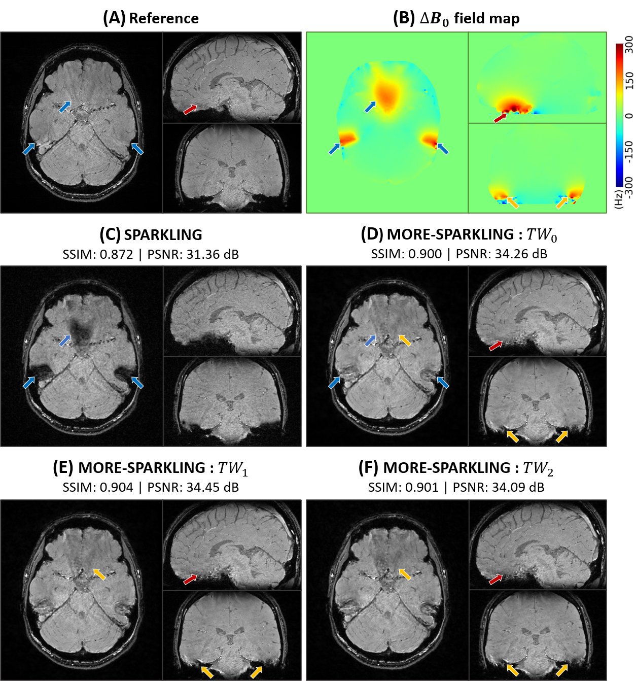
Retrospective study on healthy volunteer performed by projecting a Cartesian reference acquisition (A) and using the acquired \(\Delta B_0\) field maps (B) onto different SPARKLING trajectories : (C) Without temporal weights, (D) with \(TW_0\), (E) with \(TW_1\), and (F) with \(TW_2\). The SSIM and PSNR scores are obtained by comparison with the Cartesian reference (A). Arrows are used to point out differences related to \(\Delta B_0\) blurring (blue), contrast (yellow) and anatomical details (red).
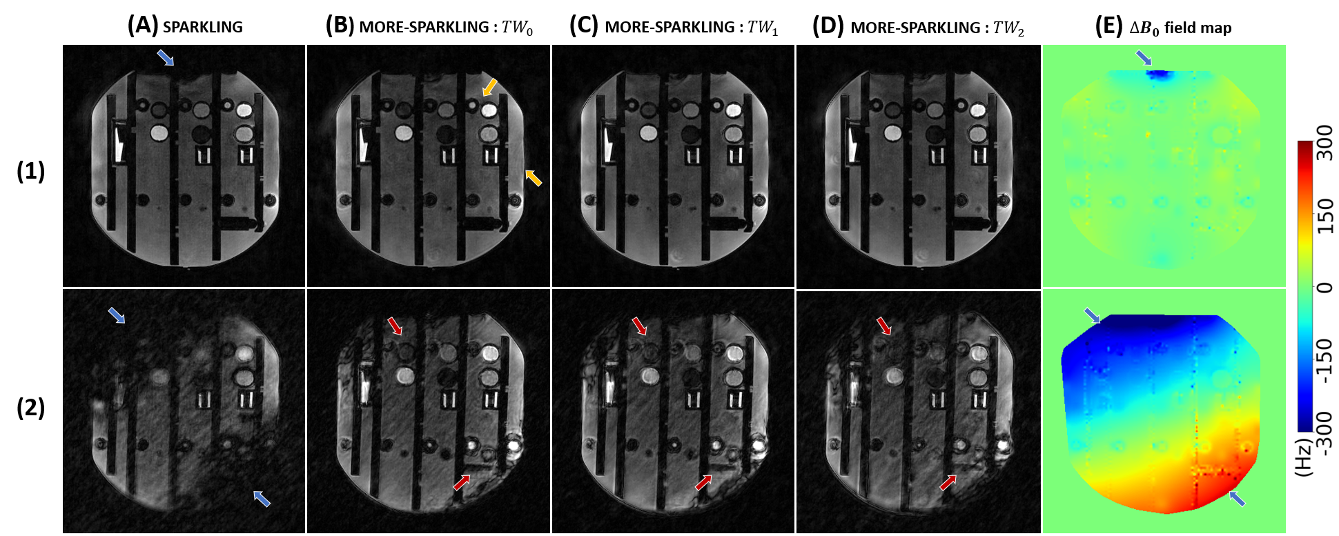
Prospective study on phantom comparing different SPARKLING trajectories : (A) Without temporal weights, (B) with \(TW_0\), (C) with \(TW_1\), and (D) with \(TW_2\). All sampling patterns are presented with (1) a complete \(B_0\) shimming and (2) with a purposely degraded \(B_0\) shimming, resulting in inhomogeneities visible on the \(\Delta B_0\) field maps (E). Arrows are used to point out differences related to \(\Delta B_0\) blurring (blue), contrast (yellow) and shape details (red).
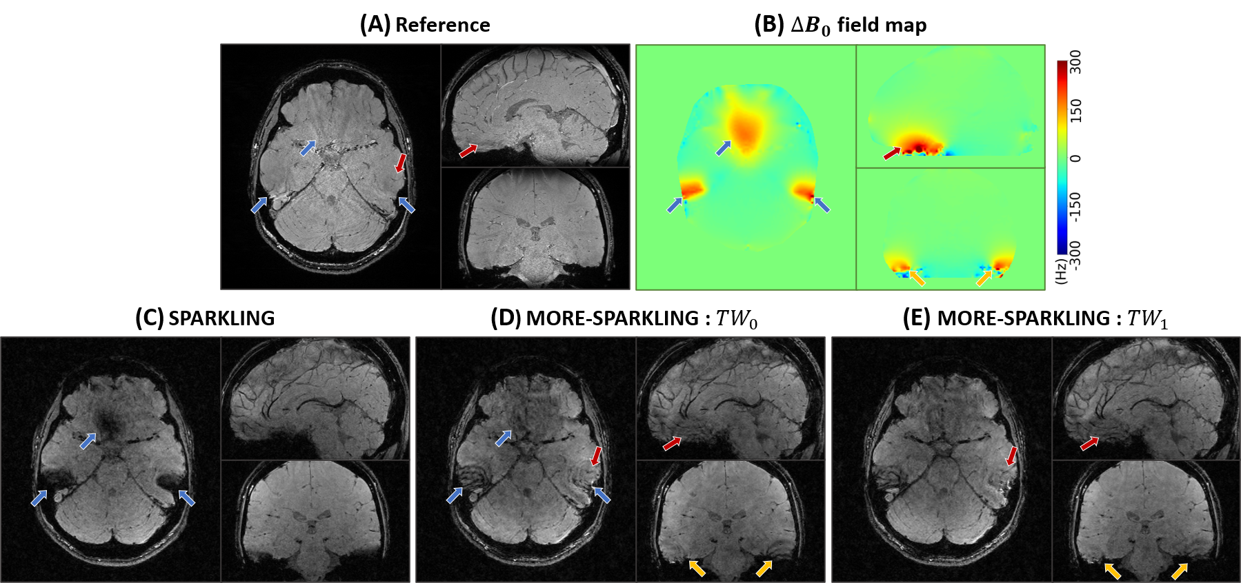
Prospective study on healthy volunteer comparing (A) a Cartesian reference with different SPARKLING trajectories : (C) Without temporal weights, (D) with \(TW_0\) and (E) with \(TW_1\). The \(B_0\) field inhomogeneities are visible on the acquired \(\Delta B_0\) field maps (B). Arrows are used to point out differences related to \(\Delta B_0\) blurring (blue), contrast (yellow) and anatomical details (red).