1585

Accuracy of quantitative DCE-MRI depends on the implementation of the convolution operation

Zaki Ahmed^1,2 and Ives R. Levesque^2,3
¹Department of Radiology, Mayo Clinic, Rochester, MN, United States, ²Medical Physics Unit, McGill University, Montreal, QC, Canada, ³Research Institute of the McGill University Health Centre, Montreal, QC, Canada

Synopsis

Quantitative DCE-MRI analysis requires fitting a model to the acquired enhancing time-course data. These models involve a convolution operation, which has a variety of possible implementations. The goal of this work was to evaluate three different implementations of the convolution operation: (i) Fourier, (ii) Summation, (iii) Iterative. The accuracy and execution time of each implementation was compared on a virtual phantom. It was found that the iterative technique was the fastest while also having the best overall accuracy.

Introduction

Pharmacokinetic modeling of dynamic contrast enhanced (DCE) MRI provides quantitative estimates of features such as blood vessel permeability and cellular density.¹ Although these quantitative features are clinically valuable, widespread adoption of quantitative DCE-MRI is hindered by poor reproducibility as different analysis software can return different results.^2,3 Some sources of variations have been studied, such as the choice of linear vs non-linear fitting^4,5 and the choice of non-linear fitting algorithm.^6–8 One factor that has not been explored is how the convolution operation inside the tracer-kinetic model is implemented. The current study evaluated three different techniques for computing the convolution operation and compared their impact on accuracy and computation time on a virtual phantom.

Methods

Theory
The current work focuses on the standard Tofts model⁹
$$c(t)=K^{trans}c_a(t)\circledast\exp(-k_{ep}\cdot t)$$
where $$$\circledast$$$ term is the convolution operator, $$$c_a(t)$$$ is the arterial input function and the fitting parameters are the transfer constant $$$K^{trans}$$$ and efflux rate constant $$$k_{ep}$$$. A third parameter—the extravascular extracellular space $$$v_e$$$—is derived via $$$K^{trans}/k_{ep}$$$.

Publicly available DCE-MRI analysis packages tend to implement the convolution operation in three ways (Table 1):
1. Fourier: By exploiting the convolution theorem, the fast Fourier transform is applied to both terms in the convolution, which are multiplied in the Fourier domain, followed by inverse Fourier transform
2. Summation: The convolution integral in the Tofts model, $$$K^{trans} \int_0^t c_a(\tau) \cdot exp(-k_{ep} \cdot (t-\tau)) d\tau$$$, is explicitly computed via numerical integration
3. Iterative: The integral form of the convolution is iteratively computed by linear interpolation, as described in the appendix of Flouri et al.⁵

Code
A potential reason for the different implementations in Table 1 could be that some languages are interpreted (MATLAB, Python), while others are compiled (C, C++, Julia), and this may influence the optimal implementation. To determine if this was a factor, all three convolution techniques were implemented in two different programming languages, MATLAB and Julia, selected for their similar syntax where one is interpreted (MATLAB) and the other is compiled (Julia).

The convolution implementations in the current work were adapted from publicly available code whenever possible. The MATLAB implementation of the Fourier technique used an in-house implementation, the Summation technique used code adapted from ROCKETSHIP,¹⁰ and the Iterative technique used code adapted from Garpebring & Löfstedt.¹¹ The Julia implementation used code adapted from DCEMRI.jl¹² for the Summation and Iterative techniques, while the Fourier technique relied on the DSP.jl package.¹³

All code used in this study is available online at: https://github.com/MPUmri/dceconv

Virtual phantom
The performance of the three convolution techniques was evaluated on a virtual phantom (ToftsV6) from the Quantitative Imaging Biomarkers Alliance (QIBA).¹⁴ This virtual phantom was simulated using a differential equation solver in JSim¹⁵ and consists of 30 unique parameter combinations, with $$$K^{trans}$$$ ranging from 0.01 to 0.35 min^-1, and $$$v_e$$$ from 0.01 to 0.5. Each voxel in the phantom contains 1321 timepoints with a temporal resolution of 0.5 seconds.

Model fitting
The Tofts model was fitted to the virtual phantom three times—each using a different implementation of the convolution operation—using non-linear least squares with the Levenberg-Marquardt algorithm. An initial guess for each parameter—required for non-linear fitting—was estimated by first fitting the linearized Tofts model with linear least-squares (LLSQ).⁴

Results

The Iterative technique was the most accurate, with percentage errors within 0.25% for $$$K^{trans}$$$ and $$$v_e$$$, while the Fourier approach was the least accurate with percentage errors exceeding 20% at some parameter combinations (Figs.1&2). The Summation approach had moderate accuracy with a maximum error of 2.1%.

The Iterative algorithm was the fastest, taking less than 60ms to fit the 30 parameter combinations in the virtual phantom, while the Summation approach was the slowest, taking over 7 seconds (Table 2). One issue with this evaluation is that the virtual phantom had 1321 timepoints which may not be realistic, so the virtual phantom was downsampled by a factor of 15 to produce 89 timepoints. The summation approach had a substantial speed improvement on the downsampled data, but it was was still 10 times slower than the Iterative approach. All times were obtained on an i5-8500 CPU by averaging 10 runs.

Discussion

Among the three convolution implementations, the Iterative approach was the clear winner in the virtual phantom as it was the most accurate while also being the fastest. It is surprising then that the Summation approach is more popular in publicly available packages (Table 1). Perhaps this is due to the Iterative approach not being as well-known or the Summation approach being easier to implement.

There was no substantial difference in the parameter estimates from MATLAB and Julia, but Julia was typically faster which is expected since it is a compiled language.

A fourth way of computing the convolution is with sliding-sums which is what MATLAB’s built-in conv() function uses. Although not shown in the results, this approach was also tested and it provided results identical to the Fourier approach.

Conclusion

The accuracy of tracer-kinetic modelling depends on how the convolution operation is implemented. This work found that the Iterative approach was the fastest and most accurate in a virtual phantom, in two languages. These results may be beneficial for researchers and clinicians that develop in-house tool for quantitative DCE-MRI analysis.

Acknowledgements

Funding for this work was provided by the Research Institute of the McGill University Health Centre (Montreal General Hospital Foundation), a NSERC Discovery Grant, the NSERC CREATE Medical Physics Research Training Network (Grant no. 432290), a FRQS Doctoral Award (ZA), and a FRQS Chercheur Boursier (IL).

References

1. Khalifa, F., Soliman, A., El-Baz, A., Abou El-Ghar, M., El-Diasty, T., Gimelfarb, G., Ouseph, R., & Dwyer, A. C. (2014). Models and methods for analyzing DCE-MRI: A review. Medical Physics, 41(12), 124301. https://doi.org/10.1118/1.4898202

2. Huang, W., Li, X., Chen, Y., Li, X., Chang, M.-C., Oborski, M. J., Malyarenko, D. I., Muzi, M., Jajamovich, G. H., Fedorov, A., Tudorica, A., Gupta, S. N., Laymon, C. M., Marro, K. I., Dyvorne, H. A., Miller, J. V., Barbodiak, D. P., Chenevert, T. L., Yankeelov, T. E., … Kalpathy-Cramer, J. (2014). Variations of dynamic contrast-enhanced magnetic resonance imaging in evaluation of breast cancer therapy response: a multicenter data analysis challenge. Translational Oncology, 7(1), 153–166. https://doi.org/10.1593/tlo.13838

3. Beuzit, L., Eliat, P.-A., Brun, V., Ferré, J.-C., Gandon, Y., Bannier, E., & Saint-Jalmes, H. (2016). Dynamic contrast-enhanced MRI: Study of inter-software accuracy and reproducibility using simulated and clinical data. Journal of Magnetic Resonance Imaging, 43(6), 1288–1300. https://doi.org/10.1002/jmri.25101

4. Murase, K. (2004). Efficient Method for Calculating Kinetic Parameters Using T 1-Weighted Dynamic Contrast-Enhanced Magnetic Resonance Imaging. Magnetic Resonance in Medicine, 51(4), 858–862. https://doi.org/10.1002/mrm.20022

5. Flouri, D., Lesnic, D., & Sourbron, S. P. (2016). Fitting the two-compartment model in DCE-MRI by linear inversion. Magnetic Resonance in Medicine, 76(3), 998–1006. https://doi.org/10.1002/mrm.25991

6. Ahearn, T. S., Staff, R. T., Redpath, T. W., & Semple, S. I. K. (2005). The use of the Levenberg-Marquardt curve-fitting algorithm in pharmacokinetic modelling of DCE-MRI data. Physics in Medicine and Biology, 50(9), N85–92. https://doi.org/10.1088/0031-9155/50/9/N02

7. Fusco, R., Irccs, G. P., Petrillo, A., & Irccs, G. P. (2014). Performances of Different Algorithms for Tracer Kinetics Parameters Estimation in Breast DCE-MRI. International Journal of Electronics Communication and Computer Engineering, 5(4), 911–916.

8. Kargar, S., Borisch, E. A., Froemming, A. T., Kawashima, A., Mynderse, L. A., Stinson, E. G., Trzasko, J. D., & Riederer, S. J. (2018). Robust and efficient pharmacokinetic parameter non-linear least squares estimation for dynamic contrast enhanced MRI of the prostate. Magnetic Resonance Imaging, 48(December 2017), 50–61. https://doi.org/10.1016/j.mri.2017.12.021

9. Tofts, P. S., Brix, G., Buckley, D. L., L Evelhoch, J., Henderson, E., Knopp, M. V., Larsson, H. B. W., Lee, T.-Y., Mayr, N. a, Parker, G. J. M., Port, R. E., Taylor, J., & Weisskoff, R. M. (1999). Estimating Kinetic Parameters From Dynamic Contrast-Enhanced T1-Weighted MRI of a Diffusable Tracer: Standardized Quantities and Symbols. J Magn Reson Imag, 10(July), 223–232. https://doi.org/10.1002/(SICI)1522-2586(199909)10

10. Barnes, S. R., Ng, T. S. C., Santa-Maria, N., Montagne, A., Zlokovic, B. V., & Jacobs, R. E. (2015). ROCKETSHIP: A flexible and modular software tool for the planning, processing and analysis of dynamic MRI studies. BMC Medical Imaging, 15(1). https://doi.org/10.1186/s12880-015-0062-3

11. Garpebring, A., & Löfstedt, T. (2018). Parameter estimation using weighted total least squares in the two-compartment exchange model. Magnetic Resonance in Medicine, 79(1), 561–567. https://doi.org/10.1002/mrm.26677

12. Smith, D. S., Li, X., Arlinghaus, L. R., Yankeelov, T. E., & Welch, E. B. (2015). DCEMRI.jl : a fast, validated, open source toolkit for dynamic contrast enhanced MRI analysis. PeerJ, 3, e909. https://doi.org/10.7717/peerj.909

13. JuliaDSP. (n.d.). DSP.jl. https://github.com/JuliaDSP/DSP.jl

14. Barbodiak, D. P. (n.d.). QIBA DCE-MRI Virtual Phantoms. https://sites.duke.edu/dblab/qibacontent/

15. Butterworth, E., Jardine, B. E., Raymond, G. M., Neal, M. L., & Bassingthwaighte, J. B. (2014). JSim, an open-source modeling system for data analysis. F1000Research, 2, 288. https://doi.org/10.12688/f1000research.2-288.v3

16. Ortuño, J. E., Ledesma-Carbayo, M. J., Simões, R. V., Candiota, A. P., Arús, C., & Santos, A. (2013). DCE@urLAB: a dynamic contrast-enhanced MRI pharmacokinetic analysis tool for preclinical data. BMC Bioinformatics, 14(1), 316. https://doi.org/10.1186/1471-2105-14-316

17. DeGrandchamp, J. B., & Cárdenas-Rodríguez, J. (n.d.). Fitdcemri. https://github.com/JCardenasRdz/fitdcemri

18. QIICR. (n.d.). PkModelling. https://github.com/QIICR/PkModeling

19. Sourbron, S. P. (n.d.). Platform for research in Medical Imaging. https://github.com/plaresmedima/PMI-0.4

20. Welch, E. B. (n.d.). Pydcemri. https://github.com/welcheb/pydcemri

21. Zöllner, F. G., Weisser, G., Reich, M., Kaiser, S., Schoenberg, S. O., Sourbron, S. P., & Schad, L. R. (2013). UMMPerfusion: an Open Source Software Tool Towards Quantitative MRI Perfusion Analysis in Clinical Routine. Journal of Digital Imaging, 26(2), 344–352. https://doi.org/10.1007/s10278-012-9510-6

Figures

Table 1: A list of publicly available DCE-MRI analysis software including DCE@urLAB¹⁶, DCEMRI.jl¹², fitdcemri¹⁷, PkModelling¹⁸, PMI¹⁹, pydcemri²⁰, ROCKETSHIP¹⁰, and UMMPerfusion²¹. The programming language and convolution technique used in each package is also included. Some packages may use a built-in function where the implementation details may not be clear. Overall, the summation approach appears to be the most popular.

Figure 1: Percentage error between the estimated Ktrans and the ground truth in the virtual phantom. The three convolution implementations (Iterative, Summation, and Fourier) are shown, along with the linear least-squares (LLSQ) approach which is included for reference as it was used as the initial guess for the other three techniques. The implementations in Julia are in the top row while the ones in MATLAB are in the bottom row. Overall, the Iterative approach had the lowest errors, while the Fourier approach had the largest errors.

Figure 2: Percentage error between the estimated ve and the ground truth in the virtual phantom. Similar to Fig. 1, the Iterative approach had the lowest errors, while the Fourier approach had the largest errors.

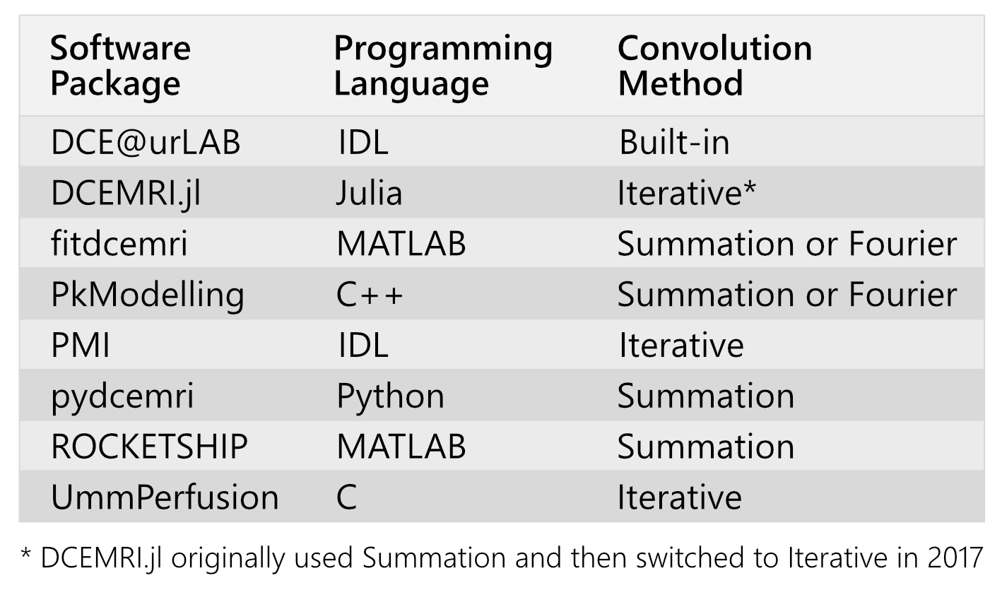
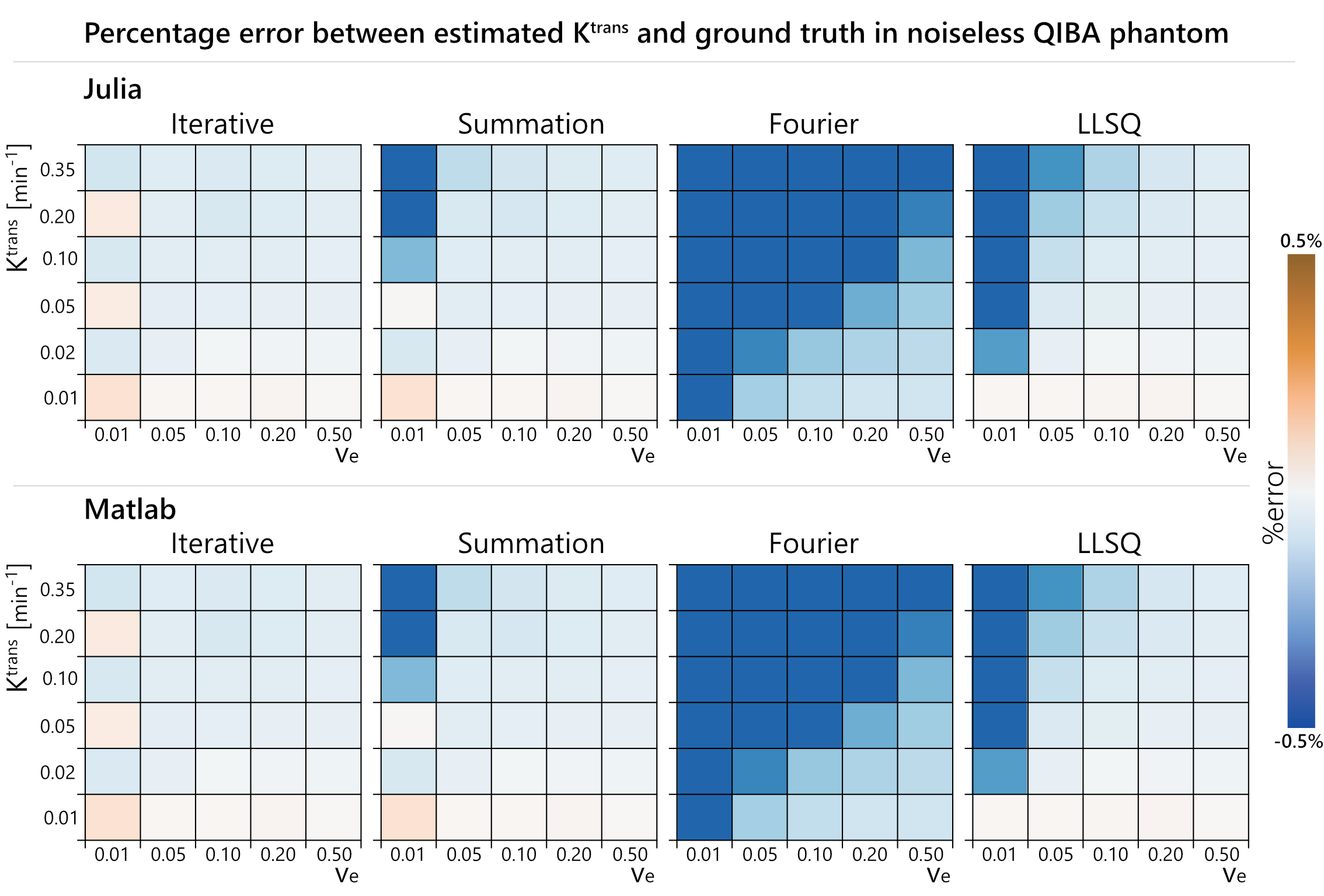
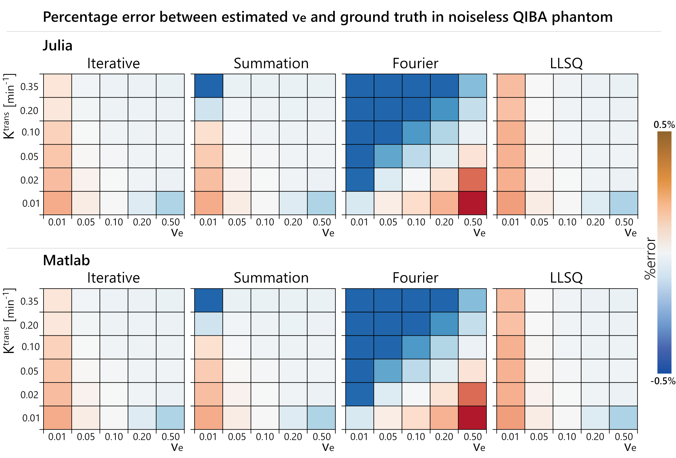
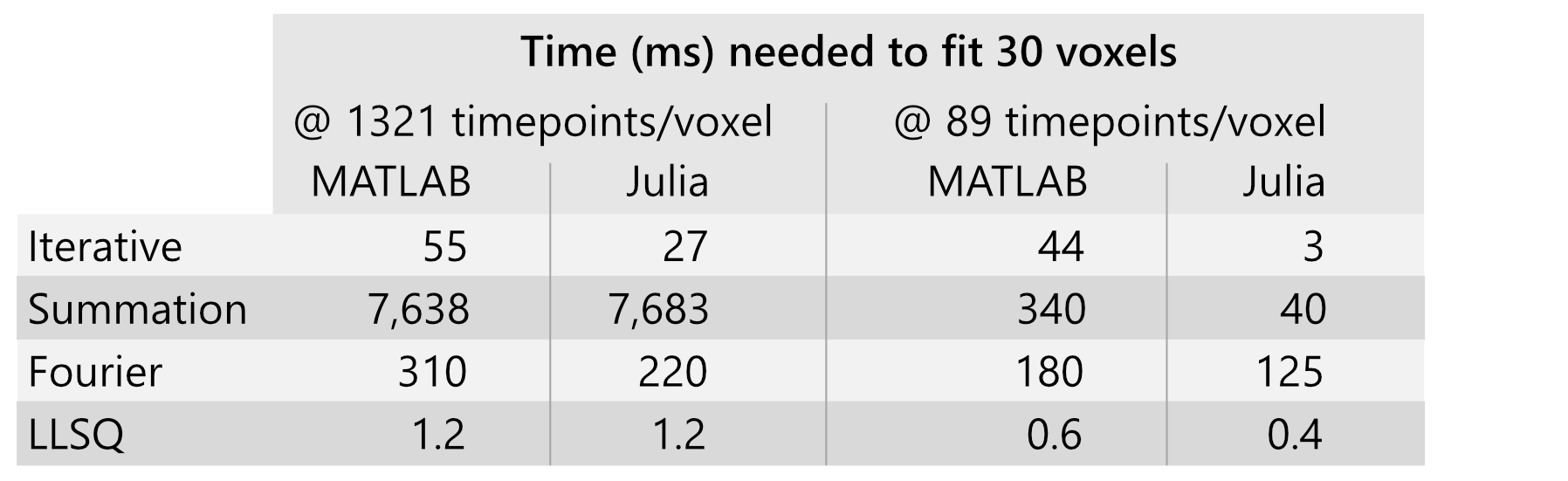
Table 2: Computation time needed to fit the 30 voxels in the original phantom which had 1321 timepoints along with the downsampled phantom which had 89 timepoints. Among the three non-linear fits (Iterative, Summation, Fourier), the Iterative approach was fastest. For reference, the linear least-squares (LLSQ) fit is included and although it is fast, it is also more sensitive to noise and temporal resolution than non-linear fitting.⁵

Proc. Intl. Soc. Mag. Reson. Med. 30 (2022)

1585

DOI: https://doi.org/10.58530/2022/1585