1580
DCE-MRI kinetic models for measuring subtle blood-brain barrier leakage– the importance of modelling finite interstitial volume fraction1Division of Neuroscience and Experimental Psychology, The University of Manchester, Manchester, United Kingdom, 2Geoffrey Jefferson Brain Research Centre, The University of Manchester, Manchester, United Kingdom, 3Faculty of Health and Medicine, The University of Lancaster, Lancaster, United Kingdom, 4Centre for Medical Image Computing, Department of Medical Physics and Biomedical Engineering, University College London, London, United Kingdom, 5Bioxydyn Limited, Manchester, United Kingdom, 6Division of Informatics, Imaging and Data Science, The University of Manchester, Manchester, United Kingdom
Synopsis
The Patlak model is commonly applied to brain DCE-MRI to quantify subtle blood-brain barrier permeability. This is based on existing evidence showing the Patlak model provides the optimal fit compared to other candidate models, including the extended Tofts model (Heye, Thrippleton et al. 2016). In this study, we compared five different tracer kinetic models in data with higher temporal resolution and determined that models which assume finite interstitial volume (ve) (e.g. extended Tofts) consistently outperform models that assume infinite ve (e.g. Patlak), particularly in gray matter.
Introduction
Dynamic contrast-enhanced MRI (DCE-MRI) is increasingly utilised to measure low-level blood-brain barrier (BBB) leakage2,3,4,5,6,7,8. The choice of model to apply is an area of active research. Heye et al.1 evaluated the fit quality of intravascular, Patlak11, and extended Tofts (eTofts)12 models in patients with small-vessel disease. In their data (Δt = 73s, 24 mins duration), the Patlak model provided the optimal fit compared to intravascular and eTofts models. Ingrisch et al.13 used higher temporal resolution data (Δt =2.1s, 7 minutes duration) but did not consider the Patlak model. They found that the two-compartment uptake (2CU) model fits best.The Patlak and 2CU models assume the interstitial volume is sufficiently large such that contrast agent does not return to blood during the measurement period. Real-time iontophoresis studies have shown the interstitial volume fraction is ~20%9, which is adequate for Patlak modelling at low leakage rates14. However, to access much of this volume, contrast agent must first navigate the perivascular space, which includes multiple diffusion barriers such as basement membranes and astrocyte end-feet. We hypothesize that for healthy BBB, or subtle BBB injury, contrast agent that leaks out of vessels may become compartmentalised in the perivascular space, leading to leakage volumes substantially smaller than 20%. Here we use high temporal resolution DCE-MRI data to evaluate suitability of different kinetic models in subjects with subtle BBB leakage. In particular, we compare models that assume infinite ve versus models that assume finite ve.
Methods
DCE-MRI data was obtained from 86 participants on a 3 T Philips Achieva scanner: healthy (n = 30), stroke (n = 15, 6-37 months post ischemic stroke), and Parkinson’s disease (n = 41). Prior to the dynamic scan, a pre-contrast T1 map was calculated from a series of 3D T1 Fast Field Echo (T1-FFE) images with flip angles 2, 5, and 10 degrees. For the dynamic series, 160 3D T1-weighted T1-FFE images were acquired with a flip angle of 10 degrees, TR/TE = 2.4/0.8ms, spatial resolution of 1.5 mm × 1.5 mm × 4 mm, temporal resolution of 7.6 s, and total duration of 20 min. On the 8th dynamic (at 60.8s), a bolus of Dotarem contrast agent of concentration 0.1 mmol/kg was administered using a power injector. Gray matter (GM) and white matter (WM) regions of interest (ROIs) were segmented on a co-registered structural 3D T1-weighted image in SPM using a probability threshold of 95%. The vascular input function (VIF) was obtained from approximately 50 voxels manually segmented from the sagittal sinus.Intravascular10, Patlak11, eTofts12, 2CU7 and two-compartment exchange7 (2CX) models were fit to mean signal from GM and WM regions of interest using least-squares curve fitting algorithm (scipy.optimize.least_squares)15 in Python (v3.8.10). To avoid local minima, start values for volume transfer constant (Ktrans) or plasma flow (Fp) were incremented (20 steps) and the fit with the lowest residual chosen. The goodness-of-fit was determined by calculating the Akaike information criterion (AIC). Paired t-tests were used to compare AIC between models. Since it is common to exclude first-pass peak data when fitting the Patlak model, fits were performed both to the entire curve and when excluding the peak, by excluding data from 0-90 s of the dynamic time series from the fit.
Results
Figure 1 and 2 show the vascular input function and model fits. The intravascular model performed the worst in all cases, predicting a much larger peak and underestimating tissue concentration at long times. The Patlak model also predicted a significantly larger peak and incorrectly predicted rising concentrations at long times. The 2CU model fitted the peak better but also predicted the same rise in tracer concentration as Patlak. Considering AIC values in Figure 3, 2CU model performed significantly better than Patlak model when the peak was included. After the peak was excluded, 2CU was only marginally better. Models that assume finite ve (eTofts, 2CX) performed significantly better than models that assume infinite ve (Patlak, 2CU) and those that assume finite ve. This difference was less pronounced in WM but still statistically significant (p < 0.05).Discussion
Our findings indicate that at high temporal resolution (Δt = 7.6 s) and scan durations of ~20 mins, the eTofts and 2CX models provide more accurate fits than Patlak and 2CU models. In particular, eTofts and 2CX models are able to more accurately describe both rapidly changing tissue concentrations occurring just after the peak and concentrations at long times. Interestingly, as Figure 4 shows, estimates of ve made using both eTofts and 2CX models were much smaller (between 3-5%) than known interstitial volume fractions (~20%), supporting our hypothesis that contrast agent is unable to access the entire extracellular space. The fact these estimates are of the order of the blood volume indicates these estimates may be a marker of perivascular space volume. eTofts and 2CX also predict Ktrans values an order of magnitude higher than Patlak, suggesting the assumption of very low leakage may not be true. Overall, our results indicate that the choice of model should be carefully considered when estimating subtle BBB leakage from DCE-MRI data, particularly when using high temporal resolution and long scan durations.Acknowledgements
We would like to acknowledge the Medical Research Council for funding the studentship of Martin Kozár.References
1. Heye, A. K., et al. (2016). "Tracer kinetic modelling for DCE-MRI quantification of subtle blood–brain barrier permeability." NeuroImage 125: 446-455.
2. Manning, C., et al. (2021). "Sources of systematic error in DCE‐MRI estimation of low‐level blood‐brain barrier leakage." Magnetic Resonance in Medicine 86(4): 1888-1903.
3. Montagne, A., et al. (2015). "Blood-Brain Barrier Breakdown in the Aging Human Hippocampus." Neuron 85(2): 296-302.
4. Montagne, A., et al. (2020). "APOE4 leads to blood–brain barrier dysfunction predicting cognitive decline." Nature 581(7806): 71-76.
5. Nation, D. A., et al. (2019). "Blood–brain barrier breakdown is an early biomarker of human cognitive dysfunction." Nature Medicine 25(2): 270-276.
6. Al-Bachari, S., et al. (2020). "Blood-Brain Barrier Leakage Is Increased in Parkinson's Disease." Front Physiol 11: 593026.
7. Sourbron, S., et al. (2009). "Quantification of cerebral blood flow, cerebral blood volume, and blood-brain-barrier leakage with DCE-MRI." Magnetic Resonance in Medicine 62(1): 205-217.
8. Tofts, P. S. and A. G. Kermode (1991). "Measurement of the blood-brain barrier permeability and leakage space using dynamic MR imaging. 1. Fundamental concepts." Magn Reson Med 17(2): 357-367.
9. Syková, E. and C. Nicholson (2008). "Diffusion in brain extracellular space." Physiological reviews 88(4): 1277–1340.
10. Sourbron, S. P. and D. L. Buckley (2013). “Classic models for dynamic contrast-enhanced MRI.” NMR in biomedicine 26(8): 1004-1027.
11. Patlak, C. S., R. G. Blasberg and J. D. Fenstermacher (1983). "Graphical Evaluation of Blood-to-Brain Transfer Constants from Multiple-Time Uptake Data." Journal of Cerebral Blood Flow & Metabolism 3(1): 1–7.
12. Tofts, P. S., et al. (1999). “Estimating kinetic parameters from dynamic contrast-enhanced T(1)-weighted MRI of a diffusable tracer: standardized quantities and symbols.” Journal of magnetic resonance imaging 10(3): 223-232.
13. Ingrisch, M., et al. (2012). "Quantification of perfusion and permeability in multiple sclerosis: dynamic contrast-enhanced MRI in 3D at 3T." Invest Radiol 47(4): 252-258.
14. Barnes, S. R., et al. (2016). "Optimal acquisition and modeling parameters for accurate assessment of low Ktrans blood-brain barrier permeability using dynamic contrast-enhanced MRI." Magnetic Resonance in Medicine 75(5): 1967-1977.
15. Eric Jones, Travis Oliphant, Pearu Peterson, et al., SciPy: Open Source Scientific Tools for Python, 2001, http://www.scipy.org/
Figures
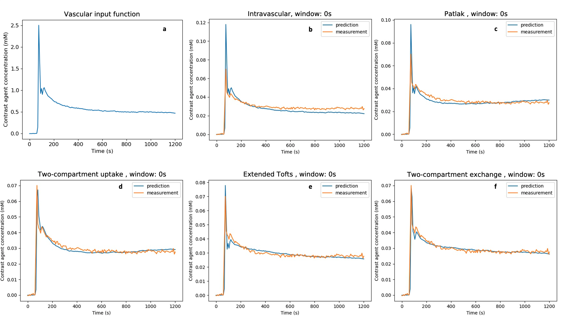
Figure 1: Model predictions when fitting to the entire measured curve (window: 0s). All plots show data from GM of a representative healthy control subject. A) The VIF B) The intravascular model gives a poor prediction for the peak and underestimates tissue concentration at long times. C) Patlak and D) 2CU have similar curve shapes, underestimating concentration just after the peak and overestimating at long times. E) eTofts and F) 2CX underestimate, overestimate, and underestimate again at short, medium and long times, but overall provide a better fit than Patlak and 2CU.
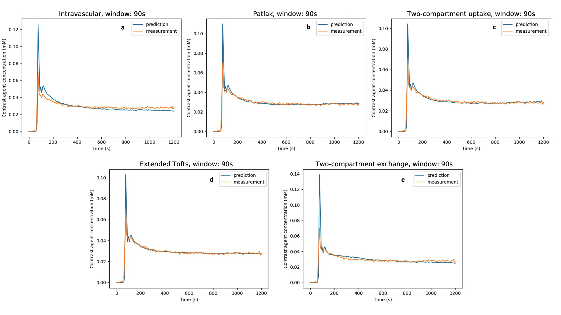
Figure 2: Model predictions when excluding the first pass peak from the fitting process (window: 90s). We observe similar behaviour as in Figure 1; however, generally the model fits are improved.
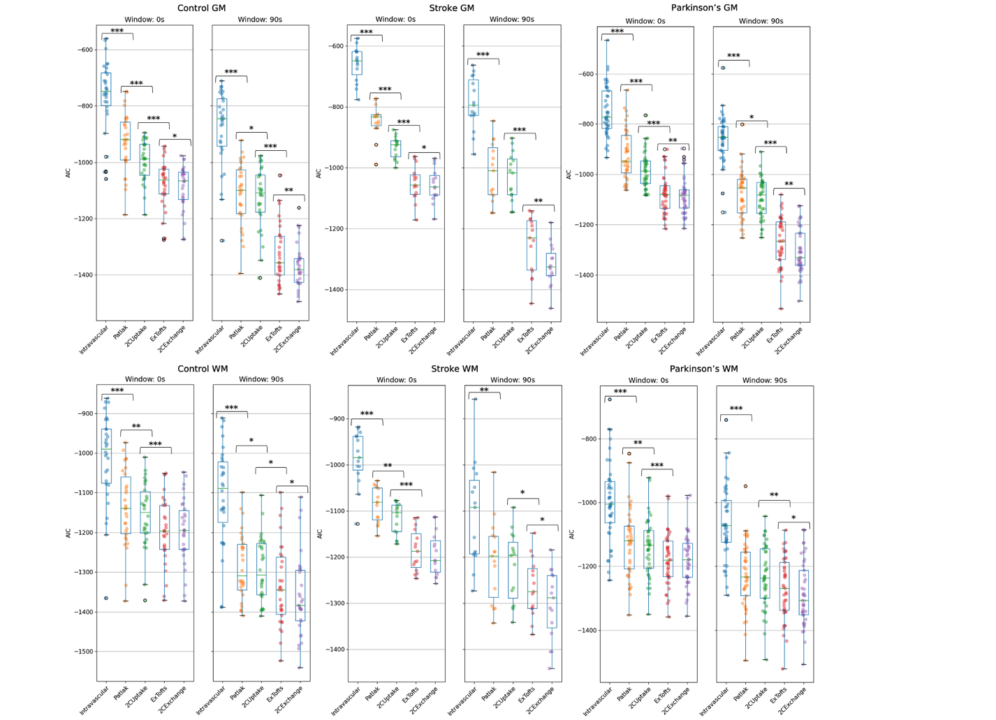
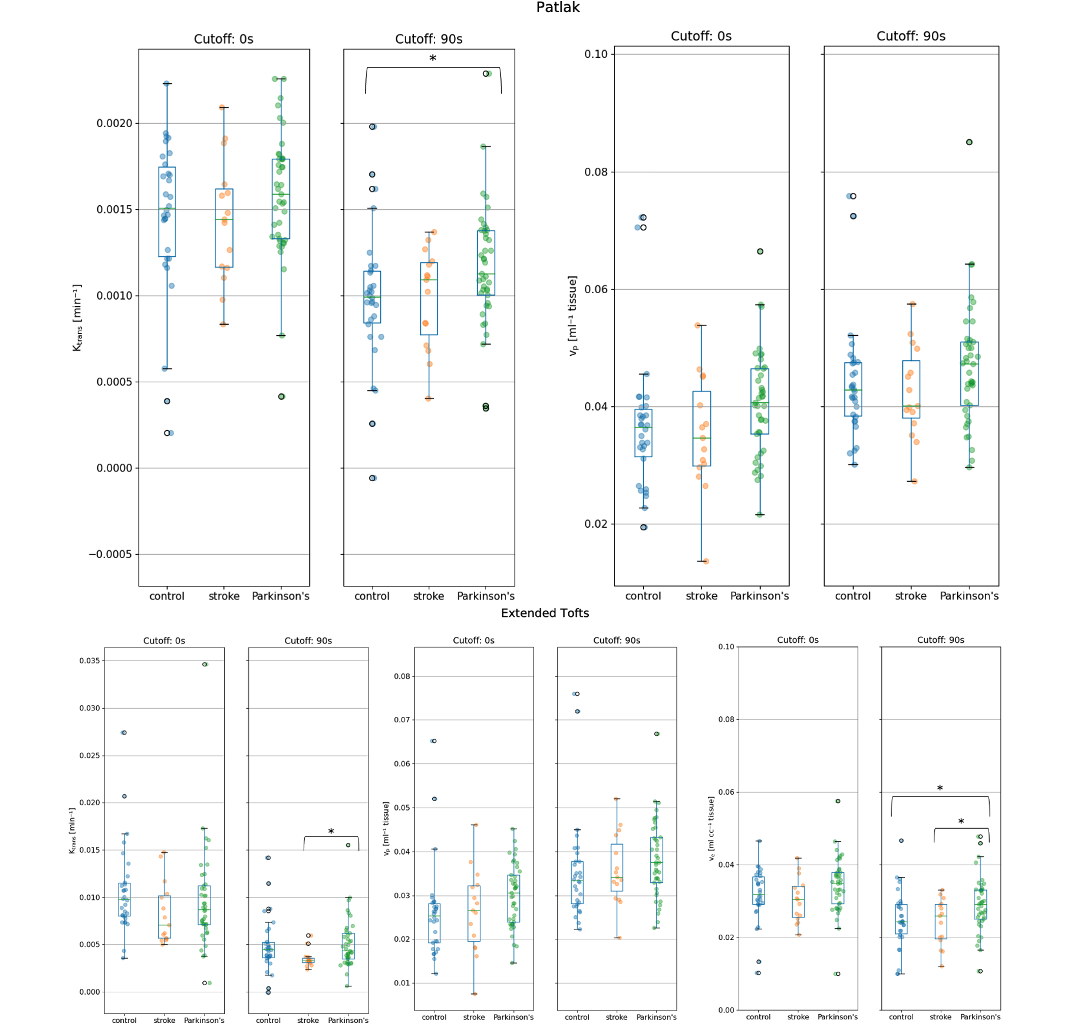
Figure 4: Estimates of kinetic parameters in gray matter. Top: Ktrans and vp for Patlak. Bottom: Ktrans, vp and ve for eTofts. eTofts predicts a Ktrans value an order of magnitude larger than Patlak. Both models predict vp values in the expected range (~3-4%). Estimates of ve from the eTofts (and 2CXM, data not shown) model are much lower (~2-4%) than known interstitial volume fractions (~20%). 1 star represents p-values between patient groups between 0.05 and 1x10⁻³.