1559
Comparison of Interpolation Methods for Ex-vivo and In-vivo Cardiac Diffusion Tensor Imaging
Johanna Stimm1, Sebastian Kozerke1, and Christian Stoeck1,2
1Institute for Biomedical Engineering, University and ETH Zurich, Zuerich, Switzerland, 2Division of Surgical Research, University Hospital Zurich, University Zurich, Zurich, Switzerland
1Institute for Biomedical Engineering, University and ETH Zurich, Zuerich, Switzerland, 2Division of Surgical Research, University Hospital Zurich, University Zurich, Zurich, Switzerland
Synopsis
To address the challenge of low resolution and limited number of slices in in-vivo cDTI, and the need for 3D structural information in image-based modeling, we compare five interpolation techniques of predominant cardiomyocyte orientation: two low-rank models, one rule-based method and two tensor interpolation approaches. The direct tensor interpolation approaches result in the smallest errors, followed by the low-rank models and the rule-based method. In view of an optimal experimental design in-vivo, the ex-vivo experiments suggest a larger benefit of increasing in-plane resolution rather than SNR, and a non-linear increase in error for less than five short-axis slices.
Introduction
Cardiac microstructure influences cardiac function. Including cardiac microstructure in computational cardiac models provides a great opportunity to understand disease progression or predict treatment outcome. In-vivo cardiac Diffusion Tensor Imaging (cDTI) allows to non-invasively measure microstructure, however, the method requires trading-off coverage of the ventricle, spatial resolution, signal-to-noise ratio (SNR) and scan time. Since biomechanical models rely on structural information on a high-resolution mesh, interpolation of cDTI data is necessary for image-based simulations. In view of optimal experimental design, this raises the question of optimal imaging settings. Therefore, we compare and analyze two low-rank models1, one rule-based method (RBM)2 and two tensor interpolation approaches3,4 to interpolate the first eigenvector of the diffusion tensor (ev1), of ex-vivo and an in-vivo cDTI data.Methods
Five porcine hearts were imaged on a clinical 1.5T MR system. Data was retrospectively collected from previous studies1,5. In-vivo imaging was performed with a second-order motion-compensated spin-echo sequence6,7. Ten consecutive short-axis slices were acquired in interleaved fashion. After fixation by retrograde perfusion under hydrostatic pressure approx. 15min after cardiac arrest, ex-vivo imaging was performed with a 3D multi-shot diffusion-weighted spin-echo sequence and EPI readout (Figure 1).The LV myocardium was segmented, and two shape-adapted coordinate systems were defined (Figure 1): Heat flux coordinates (HFC), by solving the Laplace equation with Dirichlet Boundary conditions, for each direction; Prolate Spheroidal Coordinates (PSC), by three angles relative to a truncated ellipsoid.
For the ex-vivo interpolation comparison, we generated input data with reduced resolution (1.5×1.5×8 mm3/ 2.5×2.5×8 mm3) by k-space truncation and through slice averaging, varying SNR (10;15;20;25;30) by adding Gaussian noise and reduced number of short-axis slices (3 to 9) through equidistant sampling. The ev1 was interpolated to the voxel centers of the 3D high-resolution data, providing ground truth. For the in-vivo interpolation comparison, a mid-ventricular slice was extracted to serve as reference data.
The two low-rank models1, a POD model and a PGD model using HFC, were obtained by extracting a truncated basis of the ev1 across 8 hearts (excluded from the analysis) from high-resolution cDTI data. The PGD model is based on a Proper Generalized Decomposition (PGD) within each heart and a Singular Value Decomposition across the training data. To fit the weights a modified PGD directly using the SVD basis instead of a Galerkin basis was applied. The POD model used a Proper Orthogonal Decomposition (POD) across hearts. A gappy POD8 was applied to fit the POD model.
The RBM describes the local ev1 orientation by two linear functions of transmural helix and transverse angle variation and HFC2. A least square fit of the helix and transverse angles across the data was performed. The direct tensor interpolation was performed in PSC3,4 and in HFC (IPSC/IHFC). The tensor at each target position is given by a weighted mean of the input tensors, transformed into the shape-adapted coordinates, in log-Euclidian space. The weights result from an anisotropic Gaussian kernel function and depend on the distance between input and target point and a pre-defined weighting kernel. This weighting kernel was optimized4 on one ex-vivo data set at 14 sampling points in the range of used SNR and number of slices for both resolutions. The remaining weighting kernels were approximated by a 2D second order polynomial fit.
Results
Figure 2 shows the interpolation error for the ex-vivo comparison for different input data settings of SNR, resolution, and number of slices. The tensor interpolations result in the smallest errors, followed by the low-rank models. The RBM shows the highest errors. Figure 3 depicts the error mapped onto the left ventricle (LV) for one heart. A region of elevated errors is observed at the apex for all methods. The affected area is the largest for the RBM. Figure 4 shows the interpolated ev1 for one in-vivo case. The ev1 obtained from the tensor interpolation follows the original vector field, the POD model and more severely the RBM underestimates the helix at the boundaries. Figure 5 compares the interpolation errors of the in-vivo and ex-vivo comparisons. The ex-vivo input data was chosen to match the settings of the in-vivo data. For all methods the error of the in-vivo interpolation is higher compared to the ex-vivo interpolation (case averages: (ex-vivo/in-vivo): IPSC:11.1°/12.9°, IHFC: 10.6°/13.7°, RBM: 23.9°/24.8°, PGD: 14.4°/17.9°, POD: 15.4°/19.0°).Discussion and Conclusion
The direct tensor interpolation methods show the best results with minor differences between the two coordinate systems. The low-rank models use a prior of ev1 orientation from other hearts and are less flexible when adapted to data, however, can be used as generative models. The RBM, most used in cardiac modelling, has few degrees of freedom and is not capable of capturing details of ev1 orientation leading to average errors of >23° and low sensitivity to input data quality.Higher interpolation errors in-vivo might originate from a higher data uncertainty in-vivo, supported by a similar trend when estimating the cone of uncertainty9 from the data: ex-vivo: 7.6°/in-vivo: 8.6°.
The ex-vivo experiments suggest a higher advantage of increase in in-plane resolution compared to increase in SNR of the input data (Figure 2). Reducing the number of short-axis slices below five, results in a non-linear increase in error of the 3D estimate.
Acknowledgements
This work has been supported by the Swiss National Science Foundation: PZ00P2_174144, CR23I3_166485.References
- Stimm J, Buoso S, Berberoğlu E, Kozerke S, Genet M, Stoeck CT. A 3D personalized cardiac myocyte aggregate orientation model using MRI data-driven low-rank basis functions. Medical Image Analysis 2021; 71: 102064. doi:10.1016/j.media.2021.102064
- Bayer JD, Blake RC, Plank G, Trayanova NA. A Novel Rule-Based Algorithm for Assigning Myocardial Fiber Orientation to Computational Heart Models. Annals of Biomedical Engineering 2012; 40(10): 2243–2254. doi: 10.1007/s10439-012-0593-5
- Toussaint N, Sermesant M, Stoeck CT, Kozerke S, Batchelor PG. In vivo Human 3D Cardiac Fibre Architecture: Reconstruction Using Curvilinear Interpolation of Diffusion Tensor Images. In: Jiang T., ed. MICCAI 2010. Lecture Notes in Computer Science. 6361. Springer Berlin Heidelberg. 2010 (pp. 418–425)
- Toussaint N, Stoeck CT, Schaeffter T, Kozerke S, Sermesant M, Batchelor PG. In vivo human cardiac fibre architecture estimation using shape-based diffusion tensor processing. Medical Image Analysis 2013; 17(8): 1243–1255. doi: 10.1016/j.media.2013.02.008
- Stoeck CT, Deuster vC, Fuetterer M, et al. Cardiovascular magnetic resonance imaging of functional and microstructural changes of the heart in a longitudinal pig model of acute to chronic myocardial infarction. Journal of Cardiovascular Magnetic Resonance 2021; 23(1): 103. doi: 10.1186/s12968-021-00794-5
- Stoeck CT, Deuster vC, Genet M, Atkinson D, Kozerke S. Second-order motion-compensated spin echo diffusion tensor imaging of the human heart. Magnetic Resonance in Medicine 2016; 75(4): 1669–1676. doi: 10.1002/mrm.25784
- Welsh CL, DiBella EVR, Hsu EW. Higher-Order Motion-Compensation for In Vivo Cardiac Diffusion Tensor Imaging in Rats. IEEE Transactions on Medical Imaging 2015; 34(9): 1843–1853. doi: 10.1109/TMI.2015.2411571
- Willcox K. Unsteady flow sensing and estimation via the gappy proper orthogonal decomposition. Computers & Fluids 2006; 35(2): 208–226. doi: 10.1016/j.compfluid.2004.11.00
- Jones DK. Determining and visualizing uncertainty in estimates of fiber orientation from diffusion tensor MRI. Magnetic Resonance in Medicine 2002; 49(1): 7–12. doi: 10.1002/mrm.10331
Figures

Figure 1) Workflow: I) Data
pre-processing including a) segmentation b) definition of shape-adapted
coordinates: heat flux coordinates (HFC) and Prolate Spheroidal Coordinates
(PSC); II) Application of five interpolation methods to the ev1. Two direct tensor-interpolation
approaches in HFC/PSC; a rule-based method and two low-rank models PGD/POD
model.
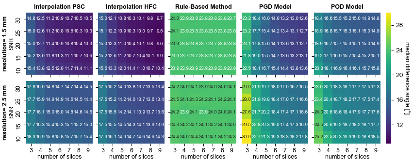
Figure 2) Ex-vivo comparison: Interpolation error as the median angular
difference between the interpolated ev1 and the ev1 from the high-resolution
ground truth data, averaged across cases. The columns represent the results
from the five interpolation methods. Each subplot shows the dependency on the
SNR and number of short-axis slices of the input data. The rows present the
results corresponding to the in-plane resolution of 1.5mm2 and 2.5mm2
of the input data.

Figure 3) Maps of the interpolation error for
one exemplary ex-vivo heart. The input data settings were: 1.5×1.5×8
mm3, SNR of 30, 7 short-axis slices, coinciding with
the settings of the in-vivo data. The columns represent the five
interpolation methods (tensor interpolation with PSC, tensor interpolation with
HFC, rule-based method, PGD model, POD model).

Figure 4) Original (grey) and interpolated ev1 field for the in-vivo
data. The mid-ventricular target slice is shown for one exemplary heart. The vectors
are color-coded according to interpolation error compared to the in-vivo ground
truth. The in-vivo input data consisted of seven short-axis slices with 2.0×2.0×8mm3
zero filled to 1.3×1.3×8mm3 resolution and SNR 30.
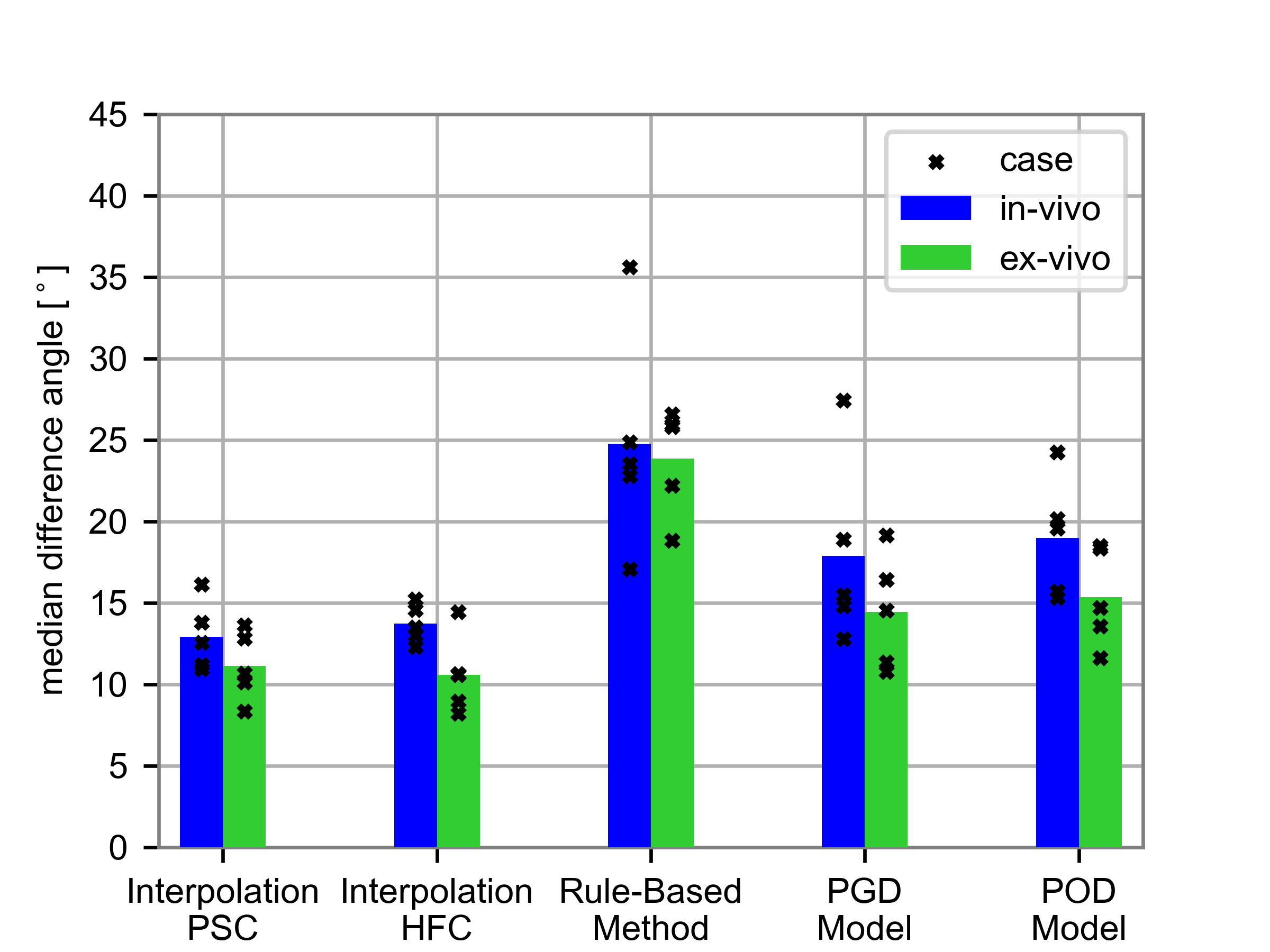
Figure 5) Comparison of the
median interpolation error averaged over the cases for the five interpolation
methods from ex-vivo (green) and in-vivo (blue) data. The markers correspond to
the individual cases. The same SNR [30(4 hearts)/25(one heart)] and number of
slices [7(3 hearts)/5(1 heart)/4(1 heart)] as in the in-vivo data and 1.5×1.5×8
mm3 resolution were considered for the ex-vivo comparison. The
location of the target data was: in-vivo: mid-ventricular slice vs. ex-vivo: 3D
LV myocardium.
DOI: https://doi.org/10.58530/2022/1559