1438
Deep Learning based Total Kidney Volume Segmentation in Autosomal Dominant Polycystic Kidney Disease1Computer Assisted Clinical Medicine, Mannheim Institute for Intelligent Systems in Medicine, Medical Faculty Mannheim, Heidelberg University, Mannheim, Germany, 2Department of Clinical Radiology and Nuclear Medicine, Medical University Center Mannheim, Medical Faculty Mannheim, Heidelberg University, Mannheim, Germany
Synopsis
The total kidney volume (TKV) increases with ADPKD progression and hence, can be used to quantify disease progression. The TKV calculation requires accurate delineation of kidney volumes which is usually performed manually by an expert physician. However, this is time consuming and automated segmentation is warranted, e.g., using deep learning. The implementation of the latter is usually hindered due to a lack of large, annotated datasets.In this work, we address this problem by implementing the cosine loss function and a technique called Sharpness Aware Minimization (SAM) into the U-Net to improve TKV estimation in small sized datasets.
Introduction
Early detection of the Autosomal Dominant Polycystic Kidney Disease (ADPKD) is crucial as it is one of the most common causes of end-stage renal disease and kidney failure. To assess disease progression is vital to plan for proper therapeutic intervention. The total kidney volume (TKV) increases with ADPKD progression and can be used in this. TKV calculation requires accurate delineation of kidney volumes which is usually performed manually by an expert, is time consuming and therefore, automated segmentation is warranted, e.g., using deep learning1. Their implementation is usually hindered due to a lack of large, annotated datasets.In this work, we address this problem by implementing the cosine loss function and Sharpness Aware Minimization (SAM) into the U-Net to improve TKV estimation in small sized datasets of only 100 samples.
Methods
Patient image data was obtained from the National Institute of Diabetes and Digestive and Kidney Disease (NIDDK), National Institute of Health, USA2,3. For this work, we selected 100 datasets of T1-weighted MRI scans of patients with different stages of ADPKD. Images were recorded in coronal orientation with a matrix of 256 x 256 and 30-80 slices with an in-plane resolution of 1.41x1.41 mm2 and slice thickness of 3.06 mm.Manual Segmentation: Two experienced physicians independently performed segmentation on the MRIs using an in-house developed annotation tool, which also allows for an analysis of the interreader agreement.
Preprocessing: The images were normalized by their mean and standard deviation and as a data augmentation technique we use a constrained label sample mining approach4, where patches are extracted from MRI slices with a patch center probability of 50:50 on label:background pixel for each batch. We train the networks on patches of size 128 x 128. For testing, we use the whole image size of 256 x 256.
Cosine loss: We adapt this loss function for the segmentation task as it has been shown to improve the image classification accuracy for small datasets5.
The loss is given by,
\[S(Y',Y)=\frac{<Y',Y>}{\parallel Y'\parallel_2 \parallel Y\parallel_2},\]
\[L_{COS}(Y' ,Y ) = 1 - S(Y', Y)\]
where S and LCOS are the cosine similarity and cosine loss, respectively between the prediction Y' and the ground truth Y .
Sharpness aware minimization (SAM): Foret et al. demonstrated that this technique helps improve the generalizability of neural networks6. Briefly, the method searches for a neighborhood of parameters with homogeneous low loss values, signifying a wide loss curve at a minimum. A wide minimum suggests that the parameters in the neighborhood will generally yield consistently better predictions compared to a minimum with a sharp curve.
Networks: All networks implemented are based on the 2D U-Net architecture by Ronneberger et al.7 extended with residual connections. For the baseline experiments, the 2D U-Net is used with Dice loss function (DSC). For training, a batch size of 8, Adam optimizer8 and a learning rate of 10-3 was used. We use exponential linear units (elus)9 as activation function with batch normalization, L2-regularization (10-7) and dropout with probability of 0.01. We perform 5 fold cross-validation with a split of 70:10:20 patient image volumes in train:validation:test sets. We select 160 samples per patient’s MRI volume during training. Networks are trained for at least 20 epochs. Thereafter, training stops if the difference in segmentation accuracy is less than 10-4 over the last ten epochs. The network’s weights with the highest average accuracy on the validation data from these last ten epochs is then selected.
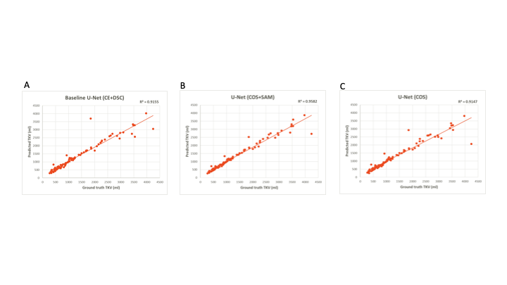
Evaluation: To compare the proposed models, we use the DSC, the mean symmetric surface distance (MSSD), and the TKV as the evaluation metrics. We compare the TKVs of the manual and the obtained segmented kidneys of our networks using scatter plots and the coefficient of determination (R2). A paired t-test is used to check for significance of obtained segmentation results. The null hypothesis (i.e. the baseline network configuration is better than the developed methods) is rejected at p < 0.05.
Results
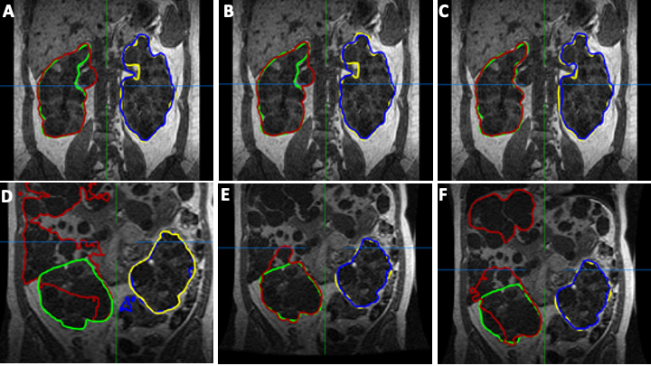
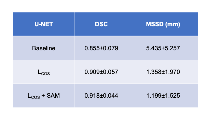
The mean interreader agreement for the manual segmentations was found to small (coefficient of variation of 0.07). Best results are obtained using the U-Net with LCOS +SAM. Here, an average DSC of 0.918±0.044 and a MSSD of 1.199±1.525 mm could be achieved. The proposed networks outperform the baseline U-Net by up to 18%. Table 1 summarizes the results. Figure 1 depicts exemplary segmentation results of the different networks. Figure 2 depicts scatter plots of manual segmented TKVs (ground truth) versus calculated TKVs from the network’s segmentations. We observe that for smaller volumes a high correlation between ground truth and segmentation exists while for larger volumes over- or undersegmentations occur. The R2 for all networks is greater than 0.91 supporting the visual analysis.Discussion & Conclusion
We demonstrated that combining the LCOS and SAM could achieve high segmentation accuracy while only using 100 datasets. Furthermore, TKV could be obtained at high accuracy compared to manual segmentation. Estimated segmentation accuracy is comparable to other approaches which used a ten-fold amount of data10,11,12. Our study shows that fast and automated segmentation and TKV estimation is possible and may allow for clinical translation in future.Acknowledgements
This research project is part of the Research Campus M2OLIE and funded by the German Federal Ministry of Education and Research(BMBF) within the Framework ”Forschungscampus: public-private partnership for Innovations” under the funding code 13GW0388A.
This project was supported by the German Federal Ministry of Education and Research (BMBF) under the funding code 01KU2102, under the frame of ERA PerMed (ERAPerMed2020-326 - RESPECT).
The Consortium for Radiologic Imaging Studies of Polycystic KidneyDisease (CRISP) was conducted by the CRISP Investigators and supported by the National Institute of Diabetes and Digestive andKidney Diseases (NIDDK). The data and samples from the CRISP study reported here were supplied by the NIDDK Central Repositories. This abstract was not prepared in collaboration with Investigators of theCRISP study and does not necessarily reflect the opinions or views oft he CRISP study, the NIDDK Central Repositories, or the NIDDK. We are thankful to the NIDDK for providing us with the patient data from theCRISP study.
We gratefully acknowledge the support of NVIDIA Corporation with the donation of the NVIDIA Titan Xp used for this research.
References
[1] Zöllner FG, Kocinski M, Hansen L et al. Kidney segmentation in renal magnetic resonance imaging - current status and prospects. IEEE Access, 2012;9:71577–71605
[2] Chapman BA, Guay-Woodford LM, Grantham JJ, et al. Renal structure in early autosomal-dominant polycystic kidney disease (adpkd): The consortium for radiologic imaging studies of polycystic kidney disease (crisp) cohort. Kidney Intl., 2003;64(3):1035–1045
[3] Niddk: Consortium for radiologic imaging studies of polycystic kidney disease (crisp). https://repository:niddk:nih:gov/studies/crisp1/, accessed:17-05-2021.
[4] A.-K. Schnurr, C. Drees, L. R. Schad, and F. G. Zöllner, “Comparingsample mining schemes for cnn kidney segmentation in t1w mri,” in 3rdIntl. Conf. Functional Renal Imag., Nottingham, UK, Oct 2019.
[5] Barz B, Denzler J. Deep learning on small datasets without pretraining using cosine loss. Proc. IEEE/CVF Winter Conf. App.Comput. Vis., 2020:1371–1380.
[6] Foret P, Kleiner A, Mobahi H et al. Sharpness aware minimization for efficiently improving generalization. Intl. Conf. Learn. Represent. (ICLR), 2021. [Online]. Available:https://openreview:net/forum?id=6Tm1mposlrM
[7] Ronneberger O, Fischer P, Brox T. U-net: Convolutional networks for biomedical image segmentation. Intl. Conf. MICCAI. Springer,2015:234–241.
[8] Kingma DP, Ba J. Adam: A method for stochastic optimization. arXiv preprint arXiv:1412.6980, 2014
[9] Clevert DA, Unterthiner T, Hochreiter S. Fast and accurate deep network learning by exponential linear units (elus),” arXiv preprint, arXiv:1511.07289, 2015
[10] Kline TL, Korfiatis P, Edwards ME et al. Performance of an artificial multi-observer deep neural network for fully automated segmentation of polycystic kidneys. J. Digit. Imaging, 2017; 30(4):442–448
[11] van Gastel MD, Edwards ME, Torres VE et al. Automatic measurement of kidney and liver volumes from mr images of patients affected by autosomal dominant polycystic kidney disease. J. Am. Soc.Nephrol., 2019;30(8):1514–1522
[12] Mu G, Ma Y, Han M et al. Automatic mr kidney segmentation for autosomal dominant polycystic kidney disease. Medical Imaging 2019: Computer-Aided Diagnosis. International Society for Optics and Photonics, 2019;10950:109500X
Figures