1416
The impact of learning rate, network size, and training time on unsupervised deep learning for intravoxel incoherent motion (IVIM) model fitting1Department of Radiology and Nuclear Medicine, St. Olav’s University Hospital, Trondheim, Norway, 2Department of Circulation and Medical Imaging, NTNU – Norwegian University of Science and Technology, Trondheim, Norway, 3Institute for Biomedical Engineering, University and ETH Zürich, Zurich, Switzerland, 4AI Medical, Zürich, Switzerland
Synopsis
We demonstrate that a high learning rate, small network size, and early stopping in unsupervised deep learning for IVIM model fitting can result in sub-optimal solutions and correlated parameters. In simulations, we show that prolonging training beyond early stopping resolves these correlations and reduces parameter error, providing an alternative to exhaustive hyperparameter optimization. However, extensive training results in increased noise sensitivity, tending towards the behavior of least squares fitting. In in-vivo data from glioma patients, fitting residuals were almost identical between approaches, whereas pseudo-diffusion maps varied considerably, demonstrating the difficulty of fitting D* in these regions.
Introduction
The intravoxel incoherent motion (IVIM)1 model for diffusion-weighted imaging (DWI) is a biexponential model composed of diffusion coefficient (D), pseudo-diffusion coefficient (D*), and perfusion fraction (F). Despite the various IVIM fitting approaches available2,3, IVIM remains challenging in the in-vivo brain due to low signal-to-noise ratio (SNR) and low F4. Recently, deep neural networks (DNN) were introduced5 as a promising alternative for IVIM fitting. Kaandorp et al.6 demonstrated unexpected correlations between the perfusion parameters with this approach, and resolved these by optimizing various hyperparameters (IVIM-NEToptim). Although IVIM-NEToptim showed promising results in the pancreas6, applying it to brain data showed poor anatomy generalization and high D* values7.In this work, we explore the impact of learning rate, network size, and training time on the convergence behavior of the unsupervised DNN loss term, and on the accuracy of the parameter estimates. We demonstrate the possible pitfalls associated with both early stopping and extensive training, using both simulations and in-vivo data from glioma patients.
Methods
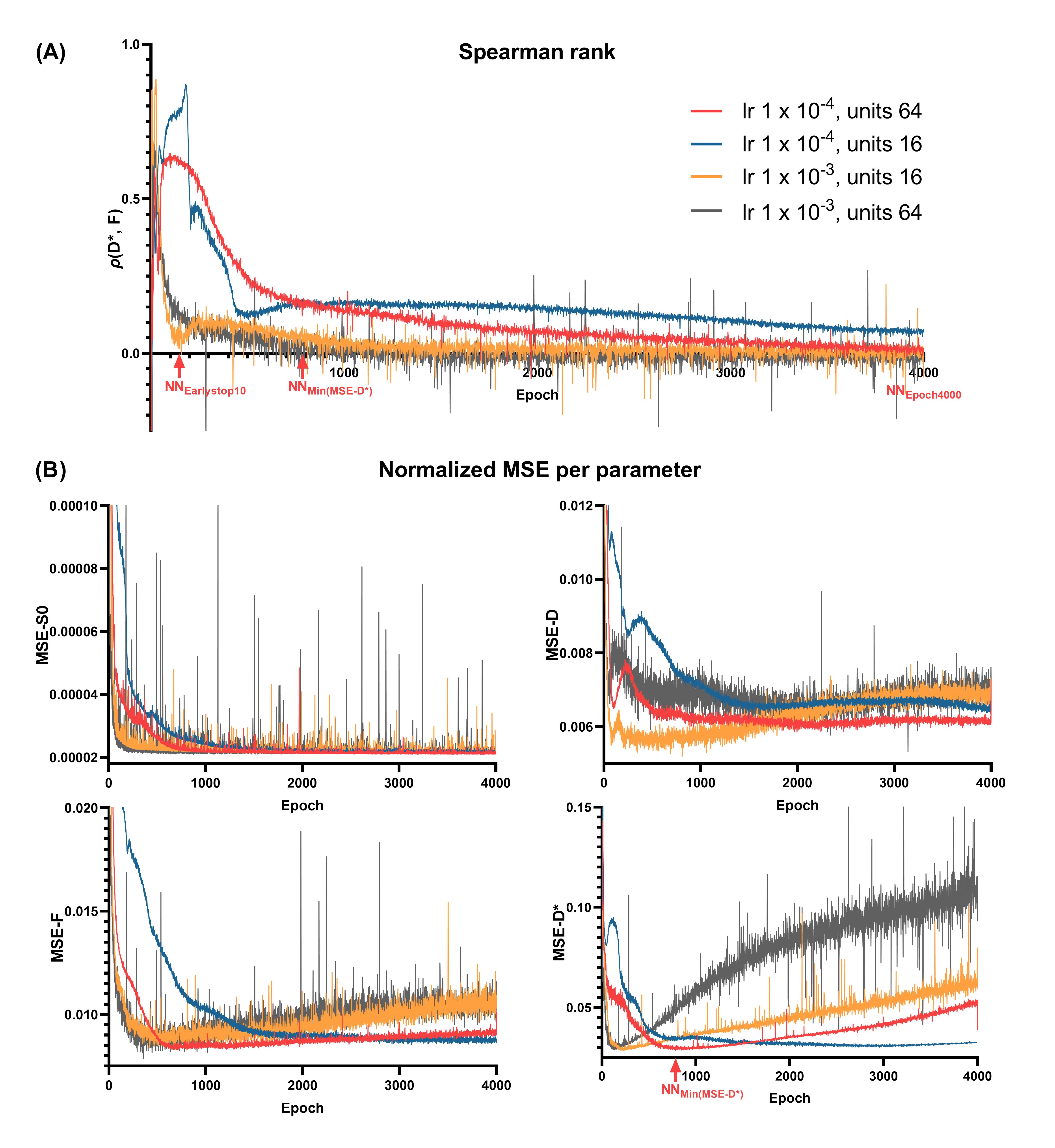
We implemented the original DNN architecture of Barbieri et al.5 in Pytorch 1.8.1. The network architecture was a multi-layer perceptron with 3 hidden layers. The network input consisted of the measured DWI signal at each b value, and the network output consisted of the three IVIM parameters plus an extra parameter S0, also considered in IVIM-NEToptim. These parameters were constrained by absolute activation functions and scaled to appropriate physical ranges (below). The network was trained using the mean-squared error (MSE) loss between the input signal and the predicted IVIM signal.Training and validation IVIM curves were simulated by uniformly sampling the parameters between: 0≤S0≤1, 0.5×10⁻³≤D≤5×10⁻³ mm2/s, 0≤F≤50%, and 10×10-3≤D*≤100×10-3 mm2/s, and considering 16 b values4. Validation data consisted of 100,000 random IVIM curves. Training was performed for 4000 epochs with 500 batches per epoch and batch size 128, similar to previous approaches5,6. Rician noise was added to the signals such that at S0=1 the SNR was 200. Four networks were evaluated by considering two different numbers of hidden units in each layer (#units = 16, 64) and two different learning rates (lr = 1×10⁻³, 1×10⁻⁴). For each network, we computed the MSE loss, Spearman’s correlation (ρ) and normalized parameter MSEs at the end of each epoch.
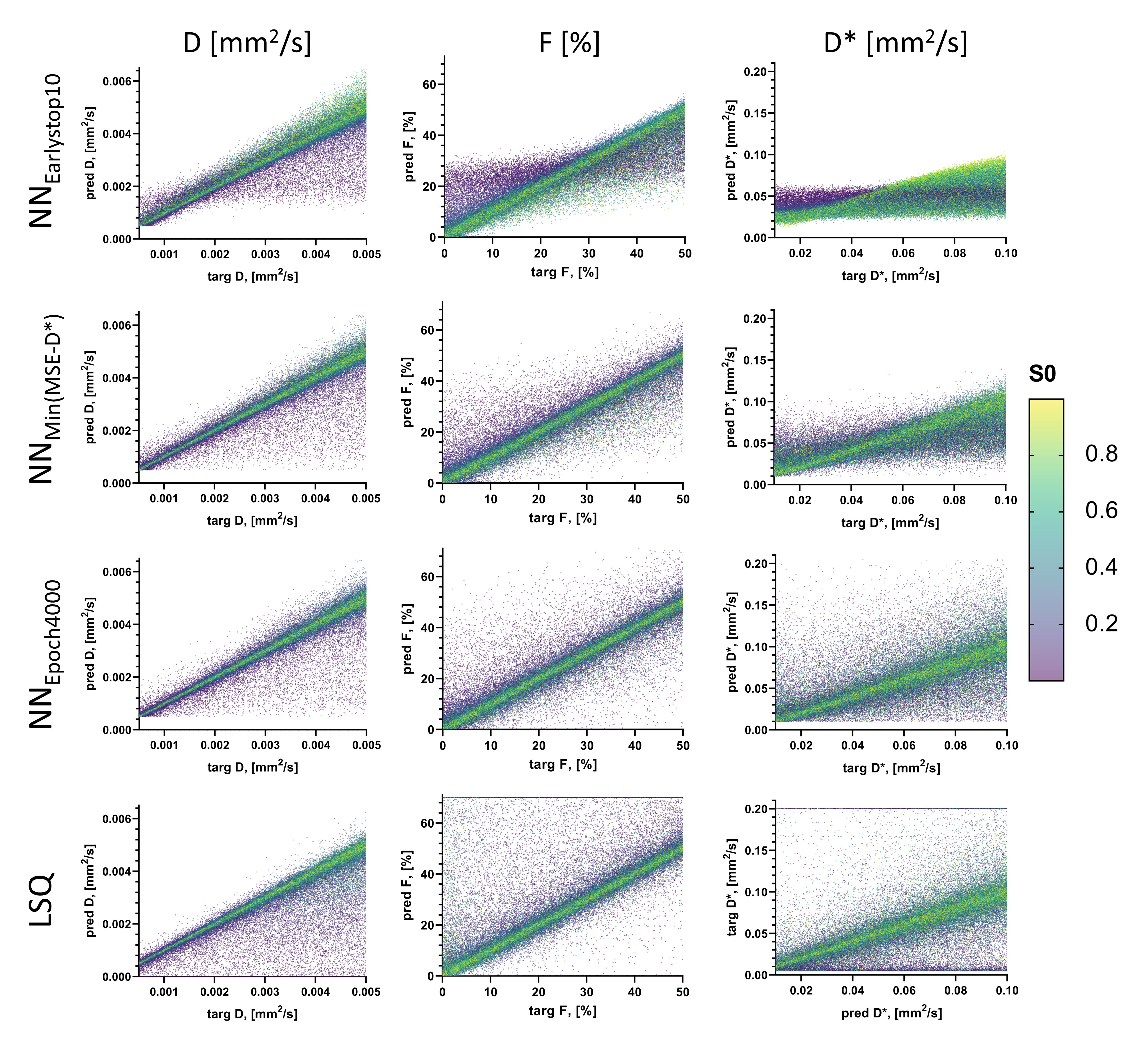
The performance of the most stable network in terms of validation convergence was evaluated by examining the distribution of individual data points in predicted-target scatter plots, and using in-vivo data from glioma patients (white matter SNR=30)4. Performance was assessed at three points during training: (i) when the validation loss did not improve over 10 epochs (NNEarlystop10), representing early stopping as used in previous approaches5,6; (ii) when MSE-D* was at a minimum (NNMin(MSE-D*)); (iii) at the last epoch (NNEpoch4000), representing extensive training. Comparisons were also made to Least Squares (LSQ) and IVIM-NEToptim.
Results
Using lower #units reduced convergence speed, whereas higher learning rate resulted in spiky convergence of the unsupervised loss term, which could result in sub-optimal solutions (Figure 1). Therefore, using #units=64 and lr=1×10⁻⁴ was considered the most stable network.The early stopping criterion (patience=10 epochs) resulted in sub-optimal solutions prior to true convergence (Figure 1), where parameters were strongly correlated (Figure 2A). Prolonging training resolved these correlations and reduced parameter MSEs (Figure 2). However, training substantially longer resulted in increased parameter MSEs, particularly for D* (Figure 2B). Figure 3 shows that at NNEarlystop10, the predicted parameters for low SNR (low S0) signals are apparently biased towards the center of the simulated distributions, particularly for D*. As training progresses, the estimates corresponding to low SNR signals exhibit higher variability and display a distribution tending towards that of LSQ.
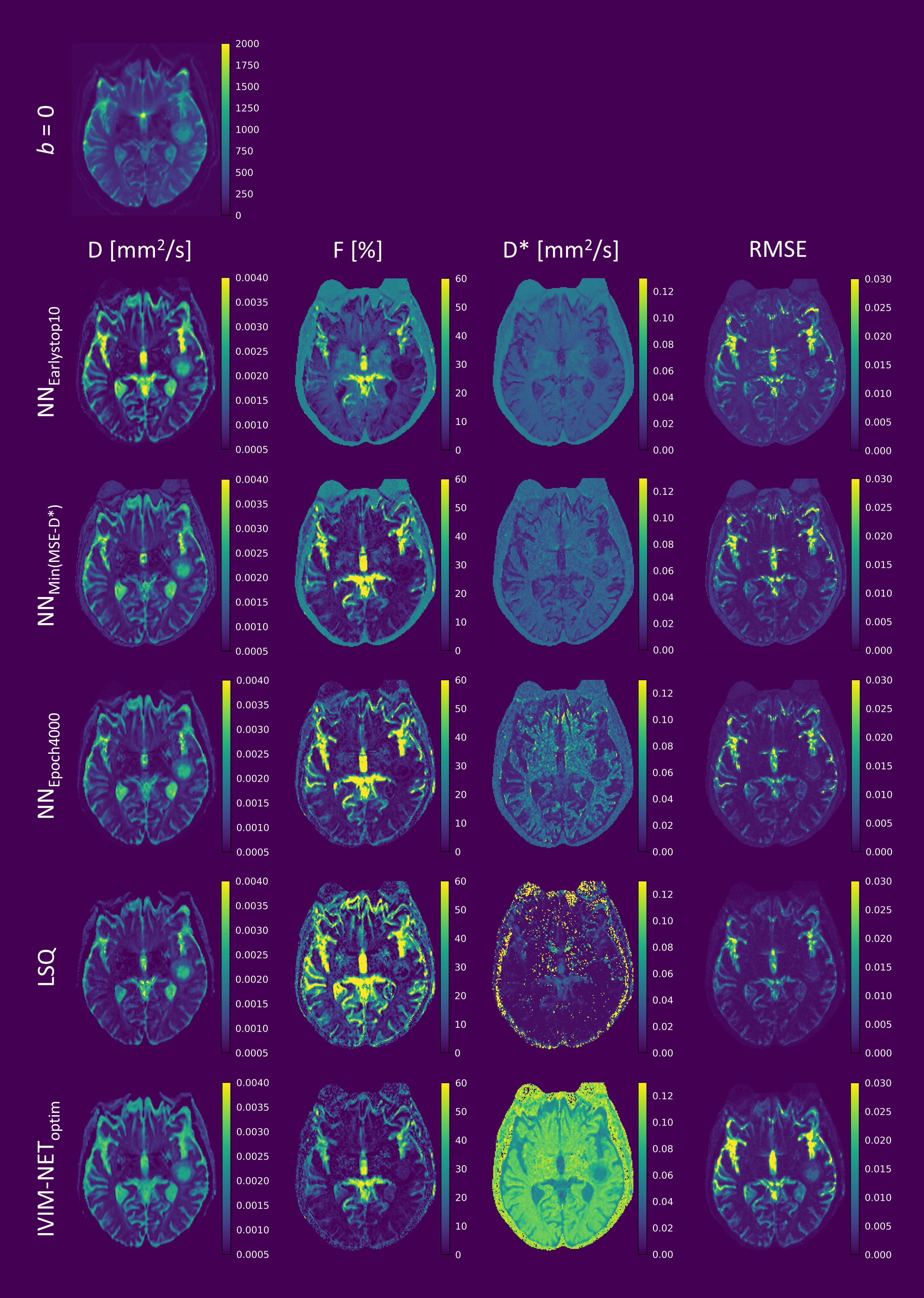
For the in-vivo data, prolonging training also improved DNN fitting and reduced root-mean-square error (RMSE), which became increasingly similar to the RMSE of LSQ as training progressed (Figure 4). However, although the RMSE-maps were similar between approaches, the D*-maps differed substantially, particularly for low SNR regions. As found in the simulations, at NNEarlystop10, the DNN tended to estimate D* towards the center of the simulated distribution, whereas prolonging training resulted in greater variability. In contrast, IVIM-NEToptim displayed inferior RMSE and high D*, as reported elsewhere for the brain7.
Discussion and Conclusion
The development of advanced estimators for IVIM modelling is often motivated by a desire to produce smoother parameter maps than LSQ, with higher accuracy and precision3. The introduction of DNNs for IVIM fitting shows promise to this end5, yet performance may be conditional on a myriad of choices regarding network architecture and training strategy6,7. In this work, we showed that high learning rate and early stopping may lead to correlated parameter estimates and sub-optimal model fitting. We showed that a lower learning rate results in more stable convergence, and extending training time leads to reduced parameter correlations and parameter error. However, extensive training resulted in an increased sensitivity to noise, somewhat akin to LSQ fitting. While this may be undesirable, it could also be argued that the corresponding variability observed in the parameter maps is indicative of the underlying uncertainty, which is indeed useful information. This uncertainty is exemplified by the contrasting D*-maps between approaches, despite the similar RMSE, and illustrates the difficulty in estimating D* in the brain.Acknowledgements
This work was supported by the Research Council of Norway (FRIPRO Researcher Project 302624).References
1. Le Bihan D, Breton E, Lallemand D, Aubin M, Vignaud J LM. Separation of diffusion and perfusion in intravoxel incoherent motion MR imaging. Radiology. 1988;168:497–505.
2. Gurney-Champion OJ, Klaassen R, Froeling M, Barbieri S, Stoker J, Engelbrecht MRW, Wilmink JW, Besselink MG, Bel A, van Laarhoven HWM, Nederveen AJ. Comparison of six fit algorithms for the intravoxel incoherent motion model of diffusion-weighted magnetic resonance imaging data of pancreatic cancer patients. PLoS One. 2018;13(4):1-18. doi:10.1371/journal.pone.0194590
3. While PT. A comparative simulation study of bayesian fitting approaches to intravoxel incoherent motion modeling in diffusion-weighted MRI. Magn Reson Med. 2017;78(6):2373-2387. doi:10.1002/mrm.26598
4. Federau C, Meuli R, O’Brien K, Maeder P, Hagmann P. Perfusion measurement in brain gliomas with intravoxel incoherent motion MRI. Am J Neuroradiol. 2014;35(2):256-262. doi:10.3174/ajnr.A3686
5. Barbieri S, Gurney-Champion OJ, Klaassen R, Thoeny HC. Deep learning how to fit an intravoxel incoherent motion model to diffusion-weighted MRI. Magn Reson Med. 2020;83(1):312-321. doi:10.1002/mrm.27910
6. Kaandorp MPT, Barbieri S, Klaassen R, van Laarhoven HWM, Crezee H, While PT, Nederveen AJ, Gurney-Champion OJ. Improved unsupervised physics-informed deep learning for intravoxel incoherent motion modeling and evaluation in pancreatic cancer patients. Magn Reson Med. 2021;86(4):2250-2265. doi:https://dx.doi.org/10.1002/mrm.28852
7. Spinner GR, Federau C, Kozerke S. Bayesian inference using hierarchical and spatial priors for intravoxel incoherent motion MR imaging in the brain: Analysis of cancer and acute stroke. Med Image Anal. 2021;73:102144. doi:https://dx.doi.org/10.1016/j.media.2021.102144
Figures