1374
A Fast Magnetostaic Inverse Approach for Subject-Specific ∆B0 Shim Coil Calibration1Department of Electrical Engineering and Computer Science, Massachusetts Institute of Technology, Cambridge, MA, United States, 2Institute for Medical Engineering and Science, Massachusetts Institute of Technology, Cambridge, MA, United States
Synopsis
For a rigidly positioned ∆B0 shim coil, calibration is a one-time process of acquiring high resolution ∆B0 fields. For subject-specific shim coil position, this approach is too slow. We propose a fast magnetostatic inverse approach for subject-specific calibration by only acquiring few, low resolution fieldmaps each with several active shim coils. Our simulation study, which included a noise model and a measured ∆B 0 test case, suggests a scan-time reduction of afactor of 170, reducing calibration time from over an hour to less than a minute with negligible impact on shim quality.
Introduction
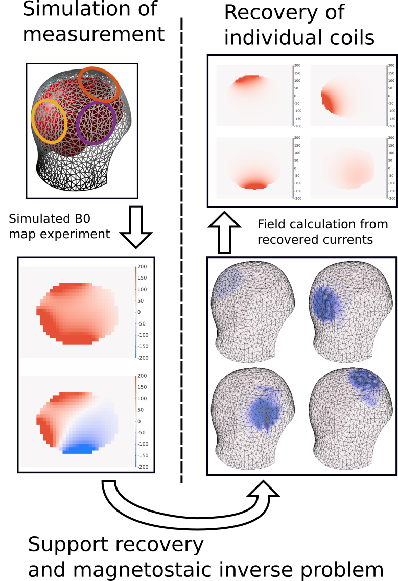
Multicoil shim-arrays for ∆B 0 field control enable a range of applications in head and neck imaging. In such applications, shim-current selection is framed as an optimization problem requiring both a fieldmap of the inhomogeneities introduced by the subject and carefully measured fieldmaps of the field produced by a known current of each shim coil. The coil field measurement process is quite long, typically requiring several hours for a 32 channel brain shim-array [1]. For a fixed shim coil geometry, the coil-specific fieldmap data is measured once.However, as the applications for ∆B0 field control expand, the possibility of subject-specific-position shim coil geometries becomes appealing and could enable new applications in body imaging [2, 3] and implant shimming [4]. The potential of non-fixed and flexible shim coils is limited by methods for rapid subject-specific shim calibration.This work presents a step in accelerating shim coil calibration in the special case that coil positions and geometry are unknown but coils are non-overlapping, and reside on a known surface. We use a magnetostatic inverse problem approach to estimate eight 2 mm resolution ∆B0 maps for each coil from three 8 mm resolution fieldmaps by acquiring calibration data while driving current through multiple coils as illustrated in figure 1.
Methods
We separate the method of shim-coil field estimation into three parts: fieldmap measurement,coil location identification and coil current refinement.We first measure ∆B0 maps while driving multiple, non-overlapping shim coils with a fixed current.
Then, in coil location identification, illustrated in figure 2, we use the fieldmaps to estimate the location of each coil on a specified surface. We compute a sparse dipole distribution on the predetermined surface that produces a magnetic field that matches our measurement by solving an l1 regularized optimization problem with ADMM [5]. We use a hierarchical clustering algorithm on the surface dipole distributions to identify the support of each coil. Coil supports are then laplacian smoothed.
In coil current refinement we solve an l1 regularized optimization problem to jointly solve for each coil’s equivalent dipole distribution, but only allow non-zero dipole distributions at the support locations for each coil computed in coil location identification.
The proposed method was evaluated in simulation of the recovery of eight 2 mm coil fieldmaps from three 8 mm simulated fieldmap measurements. Gaussian IID noise with a standard deviation of 3 Hz was added to all simulated fieldmap measurements.
Ground truth loop coil magnetic fields over the voxelized domain were calculated via Biot Savart integration. Magnetic fields due to divergence free surface currents were represented by equivalent magnetic fields due to surface-normally-oriented distributed dipole moments.The distributed dipole moments on the surface were discretized as piecewise linear distributed dipole elements centered on nodes of a triangle mesh.
Recovered field quality was evaluated by MSE from ground truth fieldmaps. Ground truth and recovered shim fields were used to calculate shim currents for an example brain homogeneity shimming case. Shim currents and shim fieldmaps were compared.
Results
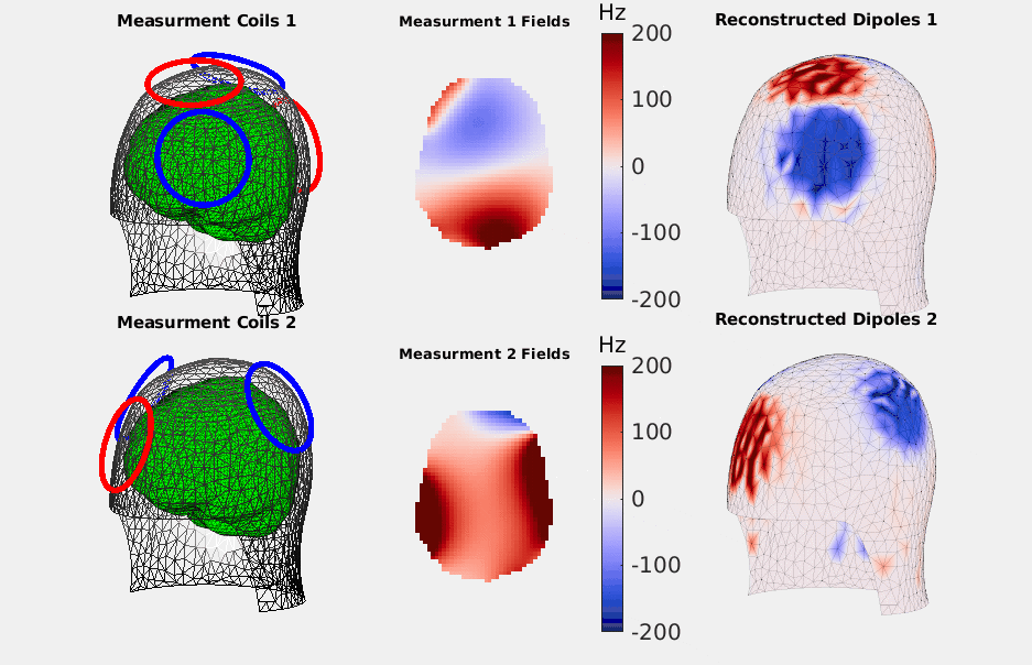
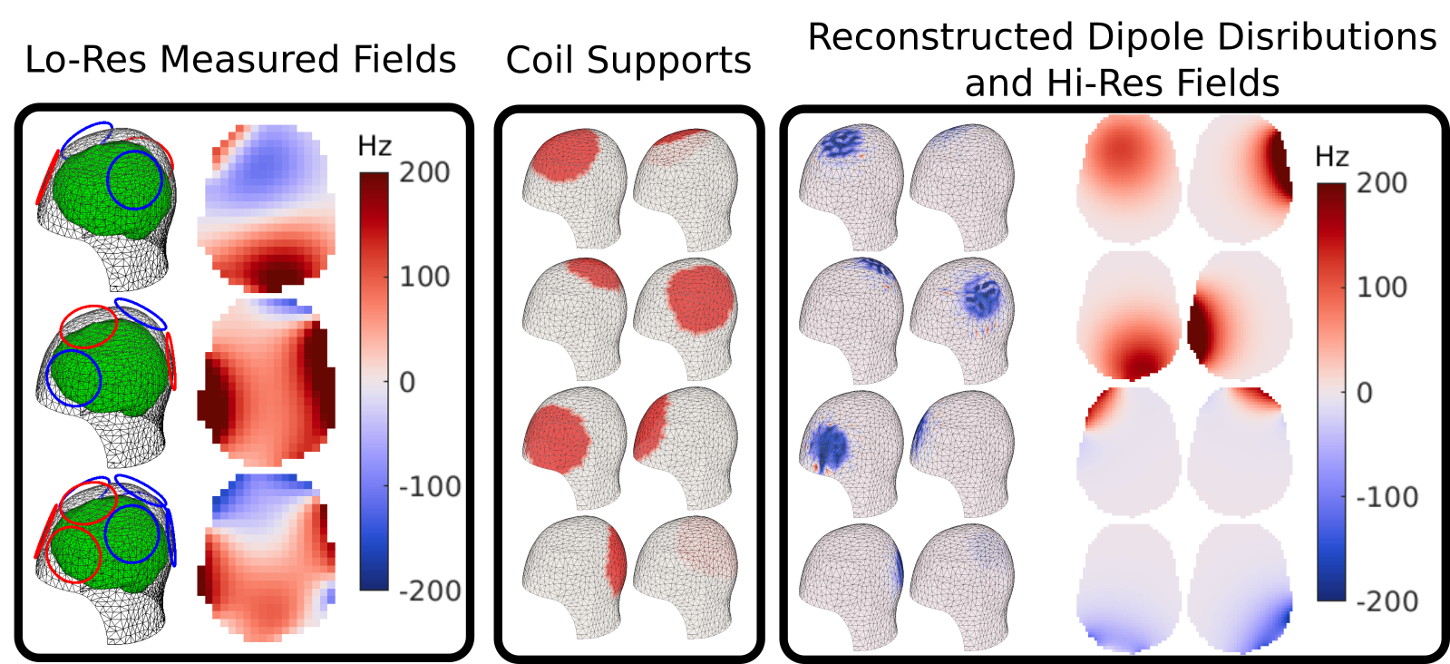
Figure 2 shows the inputs and outputs of the coil location identification step. The activated coils and their polarity are indicated with red and blue circles along with the green voxelized measurement domain. The two simulated fieldmaps from the 4-coil active states are processed with the coil location identification algorithm to reconstruct coil-equivalent sparse dipole distributions. The sparse dipole distributions are spatially compact and non-zero only in locations co-located with the active coils. Eight coil supports computed from the reconstructed dipoles are shown in figure 3. Total processing time of the location identification step was six seconds on a laptop-computer.One additional 8 mm fieldmap with all shim coils activated is used in combination with the first two fieldmaps and coil supports in coil current refinement with a total computation time of four seconds. Figure .3 shows these inputs and the reconstructed dipole distributions and ∆B0 field patterns for each of the eight reconstructed coils.
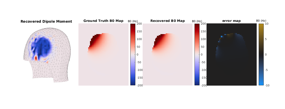
Figure 4 shows the recovered dipole moment, ground truth and recovered ∆B 0 field amps and error map from a single recovered coil. The shown recovered field has an MSE of 2.23 Hz2 over the voxelized domain, and average coil MSE was 3.52 Hz2.
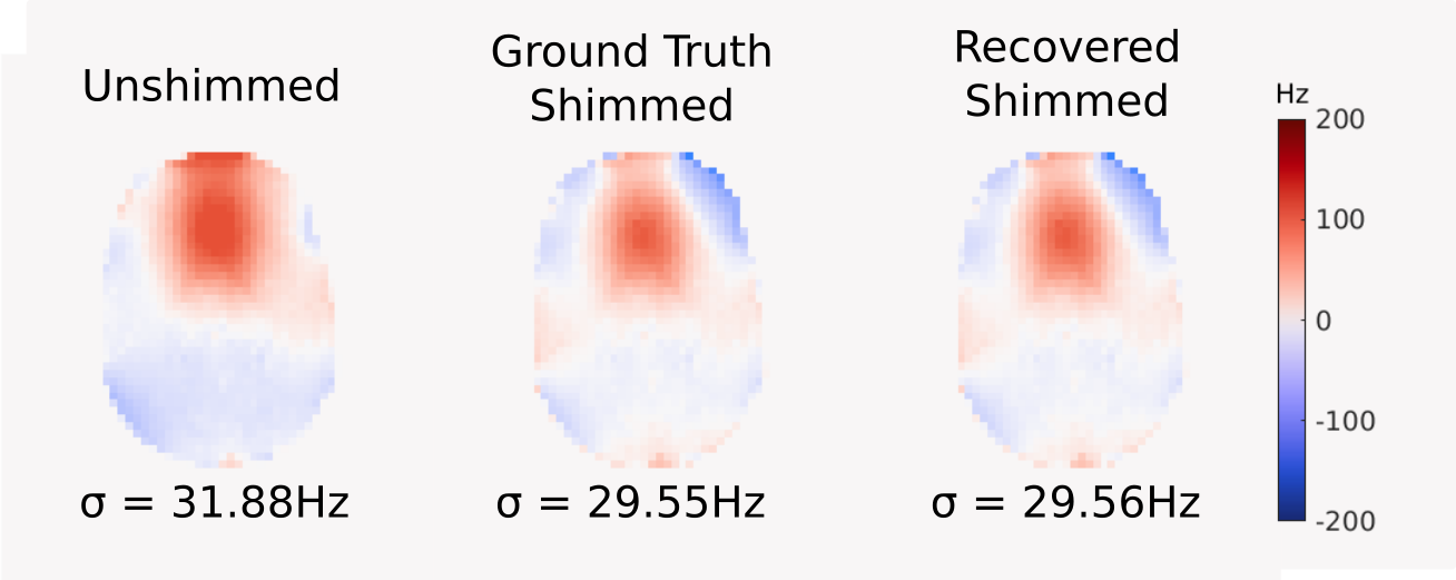
Figure 5 shows the results of the simulated ∆B0 shimming experiment. Less than 1% differencebetween shim currents computed using ground truth and recovered fields results in nearlyidentical fields, with volume standard deviations different by only 0.01 Hz.
Discussion
Our simulation study shows accurate recovery of high resolution individual shim coil fields from few low resolution fieldmap measurements with a scan time reduction 170 times (4 3 reduction in voxels and 8/3 reduction in measurements). Our highly computationally efficient methods introduce a negligible, 10 second computation after fieldmap measurement.While the technique is currently limited to sets of non-overlaping coils on a known fixed surface, future work may expand the technique to unknown smooth surfaces outside of a known body-domain to enable new opportunities for movable, subject-position-specific shim coils.
Acknowledgements
The authors thank funding support from: Next Generation Program: Skoltech – MIT Joint Projects, NIH 5R01EB006847R01EB006847References
[1] Jason P Stockmann, Thomas Witzel, Boris Keil, Jonathan R Polimeni, Azma Mareyam,Cristen LaPierre, Kawin Setsompop, and Lawrence L Wald. A 32-channel combined rf andb0 shim array for 3t brain imaging. Magnetic resonance in medicine, 75(1):441–451, 2016.
[2] Hsin-Jung Yang, Fardad Serry, Peng Hu, Zhaoyang Fan, Hyunsuk Shim, AnthonyChristodoulou, Nan Wang, Alan Kwan, Yibin Xie, Yuheng Huang, et al. Ultra-homogeneousb0 field for high-field body magnetic resonance imaging with unified shim-rf coils. 2021.
[3] Lieke van den Wildenberg, Quincy van Houtum, Wybe JM van der Kemp, Alex Bhogal,Paul Chang, Sahar Nassirpour, and Dennis WJ Klomp. B0 shimming simulations of the liver using a local array of shim coils in the presence of respiratory motion at 7 t. Tools for quantitative MR imaging and spectroscopy for the improvement of therapy evaluation in oncology, page 37, 2020.
[4] Fardad Michael Serry, Junzhou Chen, Anthony G Christodoulou, Yuheng Huang, FeiHan, Won Bae, Christine Chung, Richard Richard Handlin, John Stager, MatthewMatthew Dausch, Yubin Cai, Yujie Shan, Yucen Liu, Yibin Xie, Xiaoming Bi, RohanDharmakumar, Zhaoyang Fan, Debiao Li, Hsin-Jung Yang, and Hui Han. Improving mri near metal with local b0 shimming using a unified shim-rf coil (unic): First case study, hip prosthesis in phantom. 2021.
[5] Stephen Boyd, Neal Parikh, and Eric Chu. Distributed optimization and statistical learning via the alternating direction method of multipliers. Now Publishers Inc, 2011.
Figures