1372
Reducing MRI acoustic noise burden with Predictive Noise Cancelling
Paulina Šiurytė1, Joao Tourais1, and Sebastian Weingärtner1
1Imaging Physics, TU Delft, Delft, Netherlands
1Imaging Physics, TU Delft, Delft, Netherlands
Synopsis
Acoustic noise in MRI is a main source of patient anxiety, with noise levels reaching up to 130 dB. In this work, a low-cost solution is proposed, combining active noise cancelling and direct sequence noise prediction from the scanner gradient inputs. The prediction is based on the linearity between gradient coil input derivative and corresponding acoustic noise. A proposed Predictive Noise Cancelling demonstrated an in-bore noise reduction up to 10 dB despite the system imperfections.
Introduction
Acoustic noise in MRI is a main contributor to patient discomfort, with sound pressure levels up to 130 dB1. In addition to presently used passive earplugs or headphones, silent MRI sequences or hardware solutions have been proposed2-3. However, silent sequences often trade-off scan time or acquisition quality, and hardware upgrades are cost intensive. Active noise cancelling, i.e. using simultaneously applied anti-noise, has also been explored4, but is limited to the application of repetitive sequences only5. While this performs well in fMRI studies, clinical scan protocols contain distinct scan sequences and are therefore not suited for active noise cancelling. In this work, we present a versatile solution by combining the anti-noise approach with a direct noise prediction from the scanner gradient inputs, termed predictive noise cancelling (PNC). We describe a low cost setup for in-bore noise cancelling and evaluate its potential for noise attenuation.Methods
An acoustic setup was constructed, placing a custom speaker box and amplifier outside the scanner room and attaching a hose to channel the sound inside the bore (see fig. 1). The full setup consisted of the speaker system, optical fiber microphone (Phonoptics), function generator (Tektronix, AFG31002) and a PC for signal processing. All signals were recorded at 44.1 kHz sampling rate, filtered to 0.3-6 kHz and processed using Matlab and LabVIEW.The noise prediction was based on a linear time-invariant model, utilizing linearity between acoustic noise p(t) and the scanner gradient input derivative g`(t). In frequency domain, this is expressed as Px/y/z(f) = Hx/y/z(f) ∙ G`x/y/z(f), where Hx/y/z(f) represents a measured system transfer function6-8.
A calibration sequence was designed for a 3 T Philips system, consisting of triangular gradient pulses with a 0.14 ms rise time and 20 mT/m amplitude. 20 such blips were played out with a 3 s repetition time and used as trigger pulses (see fig. 2, black pulses). Firstly, these trigger pulses were followed by a single-gradient pulse, used to estimate the transfer functions. Next, the same pulse noise was predicted, to evaluate the maximum expected noise reduction values. Using an acoustic signal from the trigger pulses, the predicted noise was triggered to estimate the absolute latency and synchronize the system. In the final step, the anti-noise signal played out simultaneously with a scanner pulse (dashed lines in fig. 2).
Two output corrections were needed to achieve noise cancellation. Firstly, a distortion introduced by the speaker-hose system to the sound was corrected by including channel equalization. The equalizer calculates the inverse transfer function of the system from the input of the scanner pulse and a recorded playback (indicated as EQ in fig. 2). Secondly, clock mismatch between the recording device and the scanner causes the output signals to dephase. This accumulative latency was estimated based on the train of 20 trigger pulses. All recorded signals were accordingly resampled.
After the calibration steps, a prediction was applied to the components of a spoiled GRE sequence (see fig. 4, left). Theoretical maximum reduction values were estimated based on ideal equalizer and alignment conditions. The predicted anti-noise was triggered using the previously used trigger pulse. Live reduction data was acquired with 6 repetitions for each gradient coil.
Results
A clock mismatch of 12.2 μs per second was measured and used to resample the signals. The calibration pulse noise Px/y/z(f), gradient input derivative G`(f) and the derived transfer functions Hx/y/z(f) are shown in fig. 3. For the calibration pulses, estimated theoretical maximum reduction was 21 dB, assuming ideal conditions. The achieved live noise reduction for calibration pulses was 7.16 dB, 8.27 dB and 7.29 dB for X, Y and Z coils accordingly.For a spoiled GRE sequence, the estimated theoretical maxima were 9.99 dB, 13.52 dB and 9.85 dB for X,Y and Z coils respectively. Experimentally, this translated to mean values of 7.01± 0.31 dB, 6.42 ± 2.04 dB and 9.28 ± 0.26 dB reduction. An example acquisition is illustrated in fig. 5.
Discussion
Initial results with PNC using a low cost setup demonstrated noise attenuation comparable to the setting achieved in repetitive sequences or with cost intensive gradient hardware upgrades3-4.Equalizer imperfections were the main obstacle in achieving the stated theoretical estimates. Iterative equalizers can be applied for improved channel correction, and MRI compatible speakers can be employed. This will be explored in future studies to further improve noise attenuation.
Considerable noise reduction was achieved for individual gradient components. It is likely, however, that combining the gradients would result in attenuated reduction9. A segmentation of the transfer functions in terms or slew rate and/ or amplitude could help achieve stronger noise cancelling in future experiments.
Conclusion
First results of Predictive Noise Cancelling show a promise of active noise attenuation. Despite system imperfections, up to 10 dB noise reduction was presented based on a linear time-invariant prediction model, and further optimized setups may achieve even higher attenuation based on the theoretical maximum. Predictive noise cancelling, therefore, bears great promise as a cost effective solution to improve patient comfort without the need for new or modified scanner hardware.Acknowledgements
S.W. acknowledges funding from the 4TU Precision Medicine program, an NWO Start-up STU.019.024, and ZonMW OffRoad 04510011910073.References
- McJury, M. J. (2021). Acoustic Noise and Magnetic Resonance Imaging: A Narrative/Descriptive Review. Journal of Magnetic Resonance Imaging.
- Segbers, M., Rizzo Sierra, C. V., Duifhuis, H., & Hoogduin, J. M. (2010). Shaping and timing gradient pulses to reduce MRI acoustic noise. Magnetic resonance in medicine, 64(2), 546-553.
- Katsunuma, A., Takamori, H., Sakakura, Y., Hamamura, Y., Ogo, Y., & Katayama, R. (2001). Quiet MRI with novel acoustic noise reduction. Magnetic Resonance Materials in Physics, Biology and Medicine, 13(3), 139-144.
- Goldman, A. M., Gossman, W. E., & Friedlander, P. C. (1989). Reduction of sound levels with antinoise in MR imaging. Radiology, 173(2), 549-550.
- Optoacoustics, OptoActive II. https://www.optoacoustics.com/medical/optoactive-ii Accessed on November 10, 2021.
- More, S. R., Lim, T. C., Li, M., Holland, C. K., Boyce, S. E., & Lee, J. H. (2006). Acoustic noise characteristics of a 4 Telsa MRI scanner. Journal of Magnetic Resonance Imaging: An Official Journal of the International Society for Magnetic Resonance in Medicine, 23(3), 388-397.
- Sierra, C. V. R., Versluis, M. J., Hoogduin, J. M., & Duifhuis, H. (2008). Acoustic fMRI noise: linear time-invariant system model. IEEE Transactions on Biomedical Engineering, 55(9), 2115-2123.
- Wu, Z., Kim, Y. C., Khoo, M. C., & Nayak, K. S. (2014). Evaluation of an independent linear model for acoustic noise on a conventional MRI scanner and implications for acoustic noise reduction. Magnetic resonance in medicine, 71(4), 1613-1620.
- Šiurytė, P., Tourais, J., Weingärtner, S. (2021). MRI Acoustic Noise: Limits of the Linear Time-Independent Model. ESMRMB, 2021
Figures
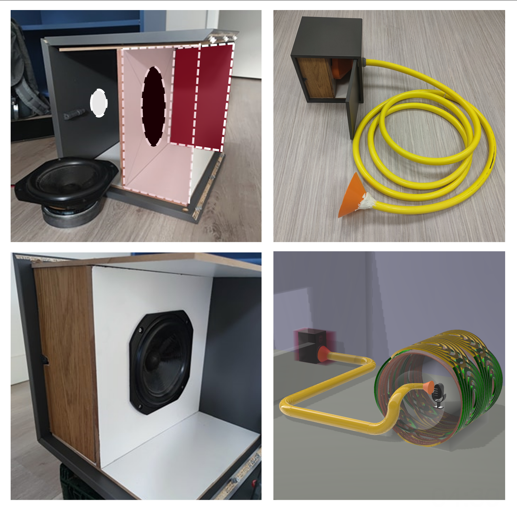
Experimental predictive noise cancellingsetup. The speaker box was constructed by placing a woofer on the left side of the wooden cabinet (top left), filling walls with acoustic wool padding and sealing it with silicon (bottom left). On the right side of the box, a funnel was fixed to attach to a rubber hose (top right), transporting the sound into the scanner room (bottom right).
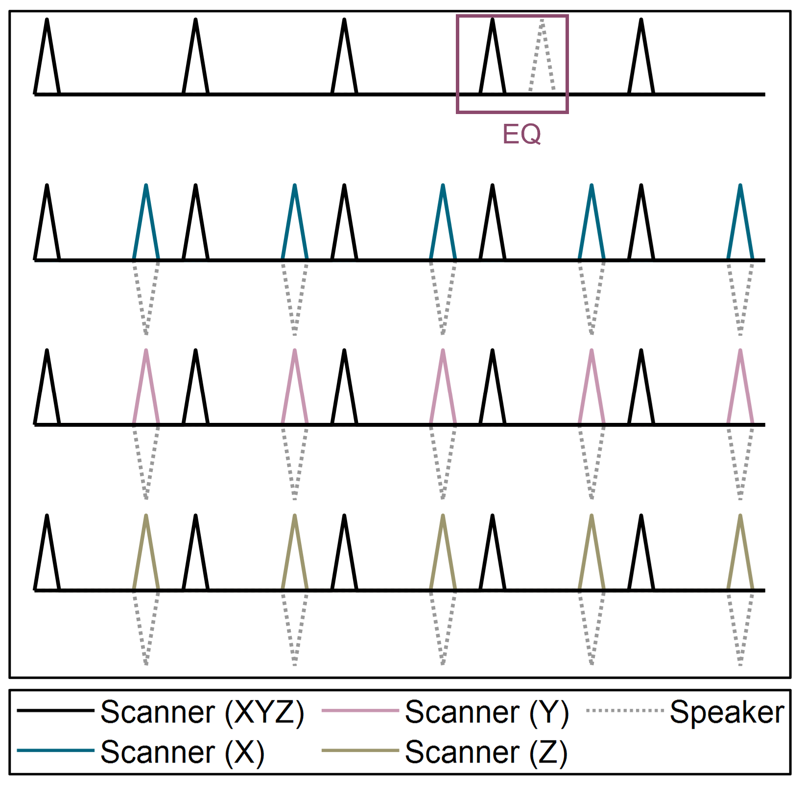
Calibration sequence scheme. All pulses have 20 mT/m amplitude and 0.14 ms rise time. Black pulses are played out on all 3 coils simultaneously, and are used as an acoustic trigger. Colored pulses represent single-gradient scanner pulses used to derive the transfer functions, while dashed lines under those indicate an anti-noise in the last calibration step. Equalizer (EQ) inputs are also indicated, where dashed pulse shows a speaker playback of the recorded trigger pulse.
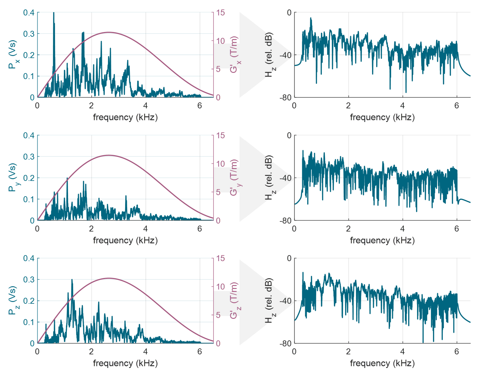
Derivation of the transfer functions Hx/y/z(f) = Px/y/z(f) / G`(f). Calibration pulse noise P(f) is illustrated on the left (blue), along with a gradient derivative G`(f) of a triangular pulse (pink). Corresponding transfer functions are plotted in relative dB scale on the right.
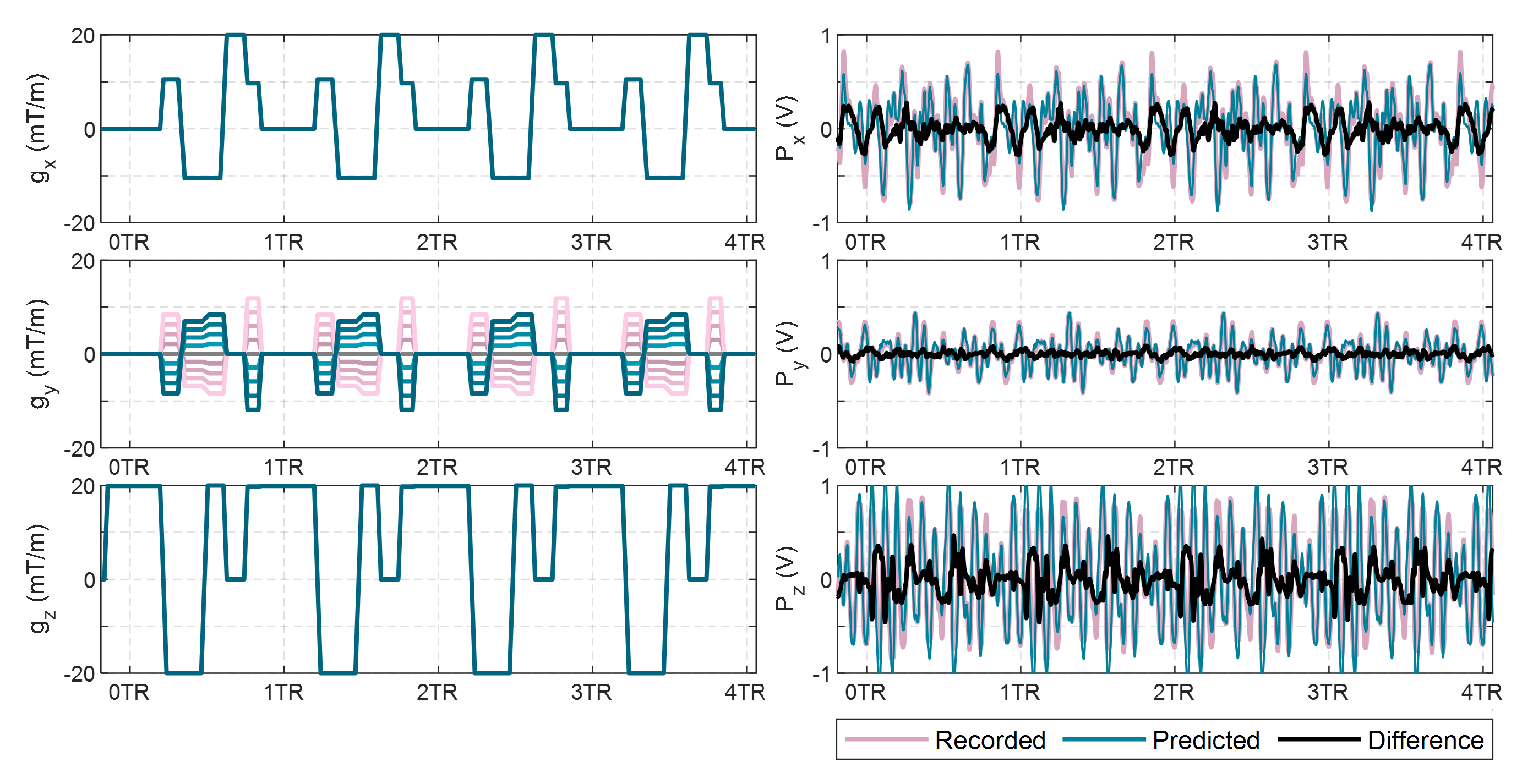
Spoiled GRE sequence gradient inputs (left). Measurement gradient was arbitrarily assigned to X coil, phase gradient to Y coil and slice selection gradient to Z coil. The corresponding noise prediction along with the original and the attenuated sequence noise is also shown (right). Sequence TR/TE = 10.6/6.4 ms ant total length - 10 s.
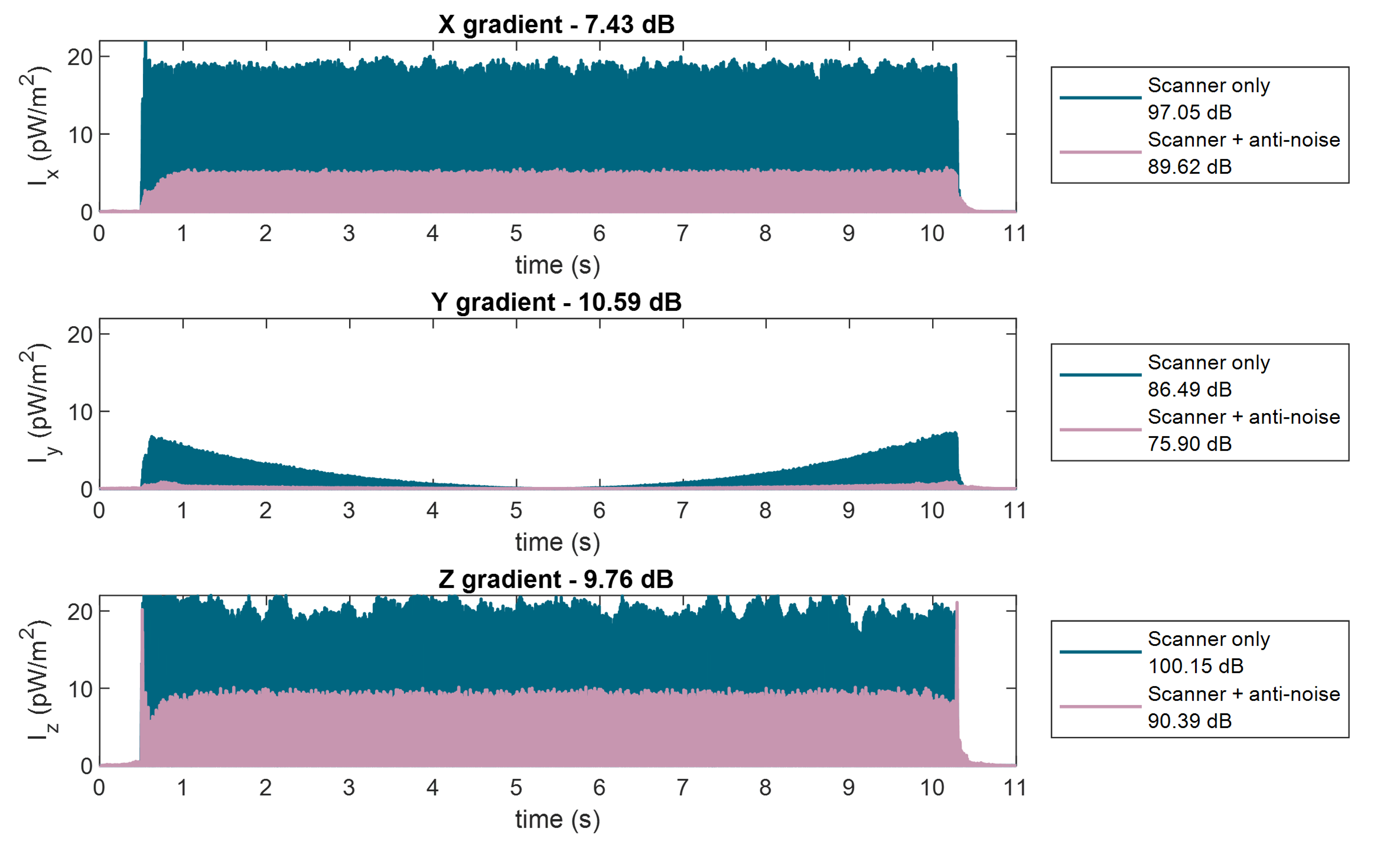
Live FFE sequence noise reduction results. Sound intensities are plotted for scanner sequence components (blue) and for scanner noise with simultaneous anti-noise output (pink). Up to 90% signal intensity reduction is shown. The reference intensity was assumed as I0 = 1 pW/m2
DOI: https://doi.org/10.58530/2022/1372