Introduction

Due to quadrupolar interactions, 23Na exhibits a bi-exponential T2 [1]. Previous approaches to estimate T2* have relied on simple least squares approaches or treating it as an inverse problem [2,3]. Both these approaches can be time consuming, and generally, solutions to inverse problems may not be unique. Here we present a fast method based on Bayesian estimation and illustrate it on an in vivo dataset.

Methods

Bayesian estimation is based on the idea of modelling the signal decomposition using a known a priori parameter distribution [4]. The sodium signal decay is simulated as a bi-exponential relaxation model using the following representation:

S = v_fexp(-t/T_f) + v_sexp(-t/T_s),

where v_f+v_s=1 and are the fractions of fast (f) and slow (s) relaxation components of sodium, respectively. The simulated signal is distorted by a non-central χ² noise (20%). The Bayesian estimation is defined as a maximisation of a posteriori probability p as x(f) = argmax p(x|f), where x is the parameter set of the relaxation model, and f are the signal features. The simulations establish the training set allowing us to find an optimised set of polynomial regressors to solve the optimisation problem. For the simulations we modelled the signal using two possible models applying either a Gaussian distribution or mixed uniform/Gaussian distribution model for the signal terms to investigate the effect of the initial distribution on the outcome of the fitting. Based on both theoretical [1] and empirical [2] evidence, we used a percent ratio of 60/40 (±20 s.d. each) for the mixing of short and long components respectively as well as 5 (±5 s.d.) ms and 20 (±10 s.d.) ms for the fast and slow component of the signal. In the uniform model, no ratio between short and long components was given. In both cases, we implied as an additional condition: v_f > v_s and T_f < T_s. A training sample size of 1 million curves was chosen.

An existing dataset from a previously published study [2] was utilised as the in vivo 23Na data and consisted of a total of 18 echo times: A multi-echo scan with 15 TEs between 0.17 and 67 ms (∆TE = 4.7 ms) and 3 additional individual scans at 0.3, 0.5 and 1 ms. Image resolution was 5 mm³ (upsampled to 3.75 mm³) and repetition time was 120 ms.

Tissue probability maps for white and grey matter (WM and GM respectively) were created in SPM (UCL, London, UK) and all processing including the Bayesian estimation were carried out in Matlab 9.5 (the MathWorks, Natick, MA).

Results

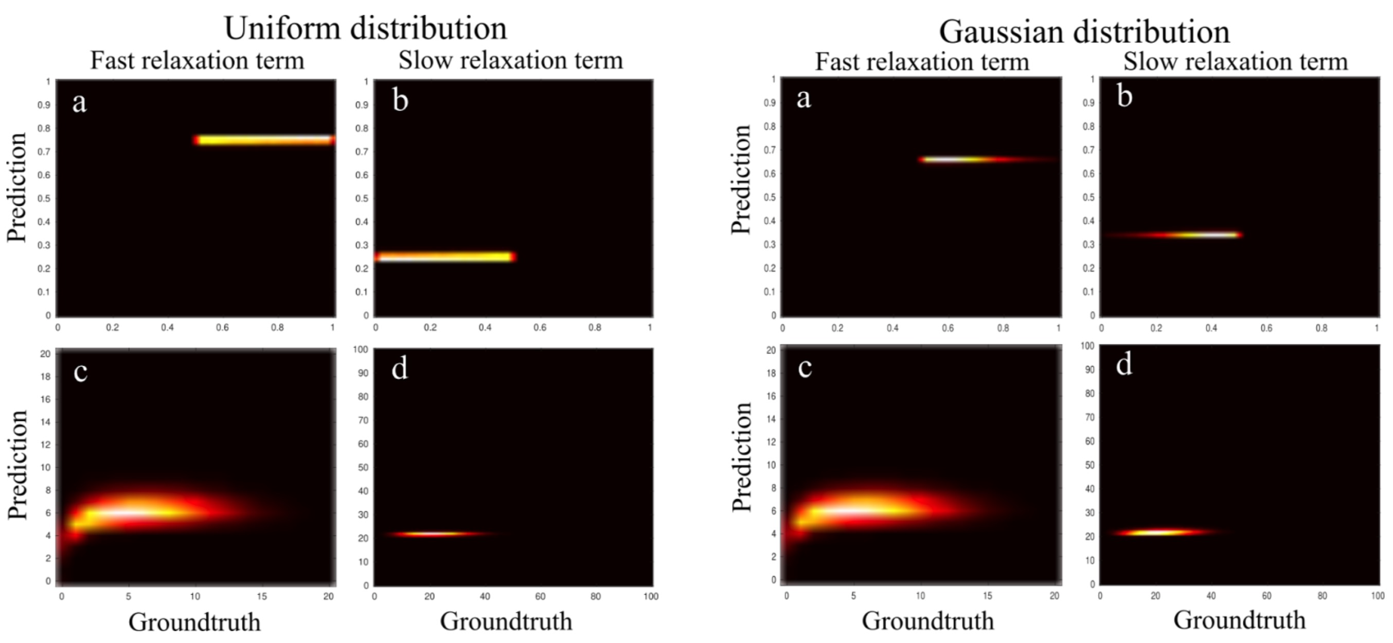
Time to perform the training (n=1.000.000 curves) and fitting of the 2.949.120 data voxels took 1.2 s on a typical consumer grade laptop (Intel i5, 4 cores) using a single-threaded process.

Figure 1 shows the results of the Bayesian model training on the simulated data. Importantly, the predicted relaxation times for both fast and slow time components are almost the same for the uniform and Gaussian fraction distributions and demonstrated a very good prediction rate.

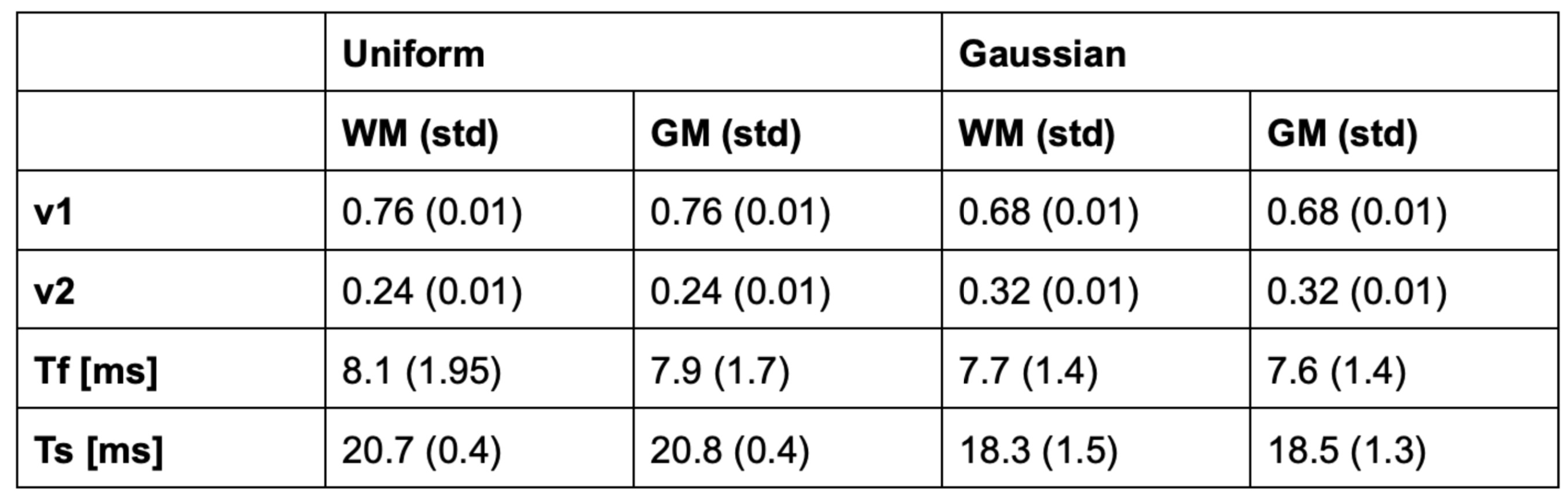
The algorithm produces a map for the volume fractions and relaxation times each. Table 1 shows summary measures extracted using tissue probability maps (>0.95) for total white and grey matter.

Discussion

Fast estimation of sodium T2* components was successfully performed. Training and estimation of relaxation parameters were performed in just over a second for a whole brain volume.

WM and GM were not significantly different from one another for v_f,v_s and T_s, but showed a trend towards a smaller short component Tf in GM. Significant difference in sodium T2* has previously been demonstrated in different regions of interest [2]. The low spatial resolution of the in vivo data and high partial volume effect probably did not allow us to demonstrate a high contrast between bulk WM and GM in the brain.

Compared to previous studies, the T_f of WM and GM was larger in our experiment, while T_s was smaller. It needs to be investigated whether this was due to the choice of training parameters and whether T_s compensates for T_f. Volume fractions v_f,v_s have rarely been reported, but were shown to vary considerably between different regions of interests but not necessarily between WM and GM using an inverse Laplace transform [2]. It is however further investigation necessary to make sure that volume fractions are captured accurately.

Using a uniform as opposed to a Gaussian distribution did not affect estimated T_f and T_s significantly, but had a stronger effect on the volume fractions v_f and v_s.

In future, we plan to develop a strategy to find the optimal training parameters with an iterative procedure and test it on a numerical T2* phantom in simulation to investigate the effects of training parameters, resolution and SNR on contrast in the maps for v_f,v_s,T_f and T_s.

Characterisation of sodium T2* may be able to disentangle cellularity changes in cancer and neurological diseases. The presented method could be used to create fast T2* maps in in vitro models where the lengthy MR acquisition protocols required for multi-echo based T2* mapping is not an issue.

Acknowledgements

F.R. is supported by a project grant from the Trond Mohn Foundation (TMF).