1283
Variability in Brain Sodium Total Sodium Content (TSC) Mapping Quantification Methods1School of Biomedical Engineering, McMaster University, Hamilton, ON, Canada, 2Imaging Research Centre, St. Joseph's Healthcare, Hamilton, ON, Canada, 3Radiology, University of Colorado Anschutz Medical Campus, Aurora, CO, United States, 4Electrical and Computer Engineering, McMaster University, Hamilton, ON, Canada
Synopsis
Throughout the literature, the methods of quantifying total sodium concentration (TSC) brain maps vary. Some studies use a two calibration phantom approach, some use a one calibration phantom approach, and some use anatomical references to quantify the TSC maps. This abstract investigates the variability of using one method versus another to see if a chosen method will inherently bias the resultant maps. It was found that no bias is provided by one method versus another as they provide no significant variance to the data.
Introduction
Throughout cerebral sodium MRI literature, the methods of quantifying the resultant total sodium concentration (TSC) maps vary. Some studies create concentration curves using two calibration phantoms of known concentrations1, others use a single phantom2, and some use anatomical regions of known sodium concentrations as the references3. This raises the question of reliability; which method – if any – provides the least amount of variability patient to patient, scan to scan?Methods
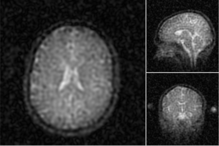
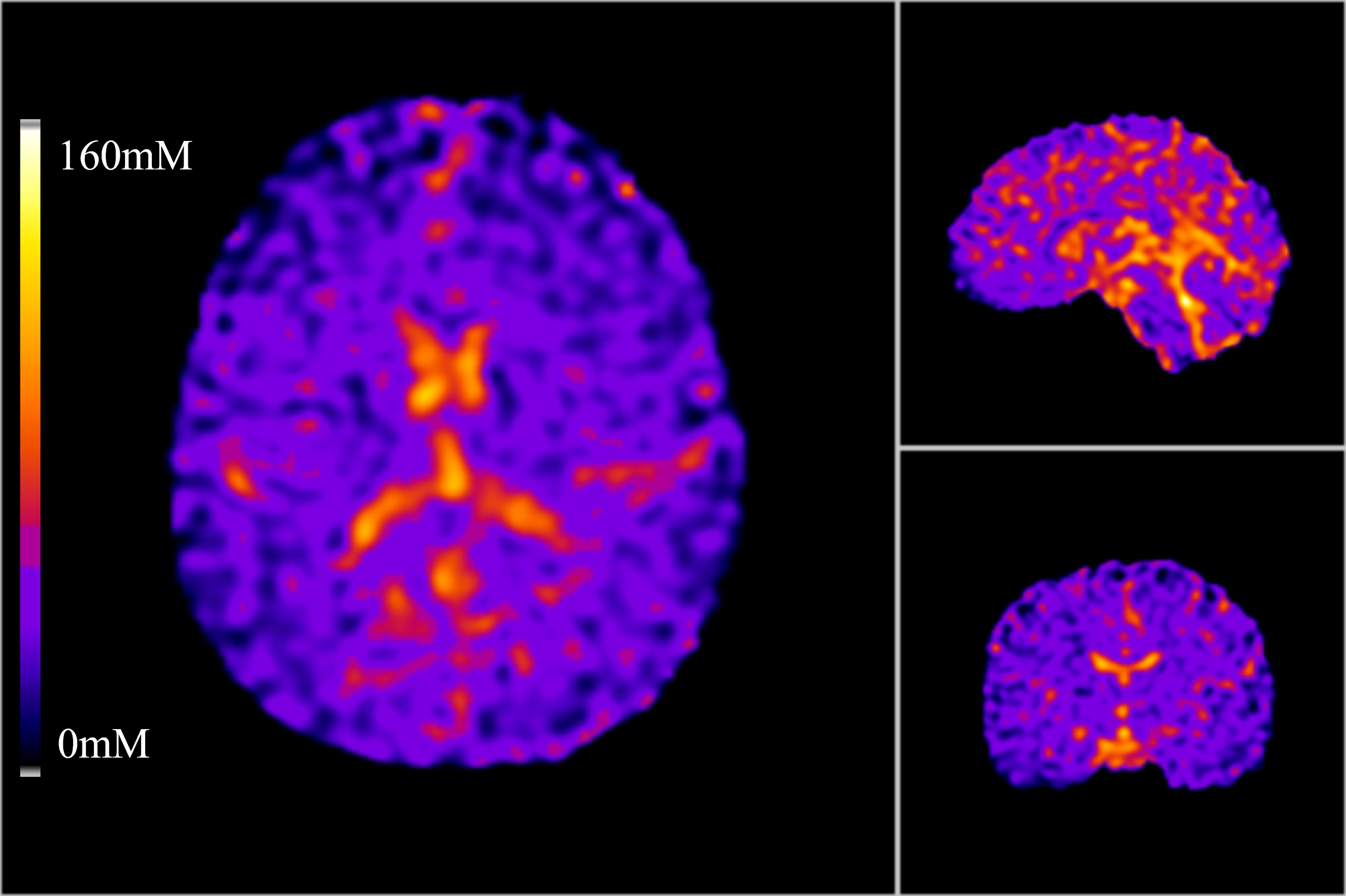
Sodium maps were created using the variable flip angle (VFA) method4 by acquiring two 3D density adapted radial projections (DA-3DRP) (0.6ms hard pulse, TR=24ms, TE=0.2ms, 240mm FOV with 3.2mm isotropic resolution) at flip angles of 70° and 30° to meet SAR constraints5. A B1+ map was also acquired using a Bloch-Siegert approach6 to correct the resultant sodium images. For registration and segmentation purposes a T1-weighted anatomical proton 3D-FSPGR (θ=12°, TR=11.4ms, 240mm FOV) was also acquired. All scanning was performed on a 3T GE MR750 (GE Healthcare, WI). The sodium reconstruction was performed using the Berkely Advanced Reconstruction Toolbox’s (BART)7 non-uniform fast Fourier Transform (NUFFT), and the TSC maps were calculated using Python 3.10 (https://www.python.org/).Two 50mL calibrants of 30mM and 80mM NaCl (in 3% agar) were included in the coil’s FOV alongside the subject being imaged. Four subjects (3 male, aged 27 ± 4.5) were scanned between 5 and 7 times over two weeks using the VFA protocol, resulting in 5 to 7 TSC maps per subject. Each map was the quantified using three methods: a linear concentration curve using the 30mM and 80mM calibrant tubes as reference, a linear concentration curve using the vitreous humor (140mM) and corona radiata (38mM) as reference, and finally simply using the single 80mM calibrant as a reference.
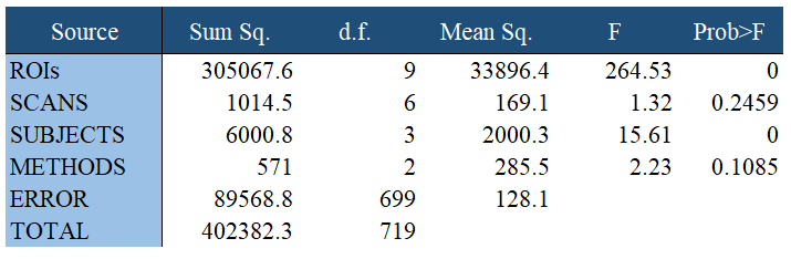
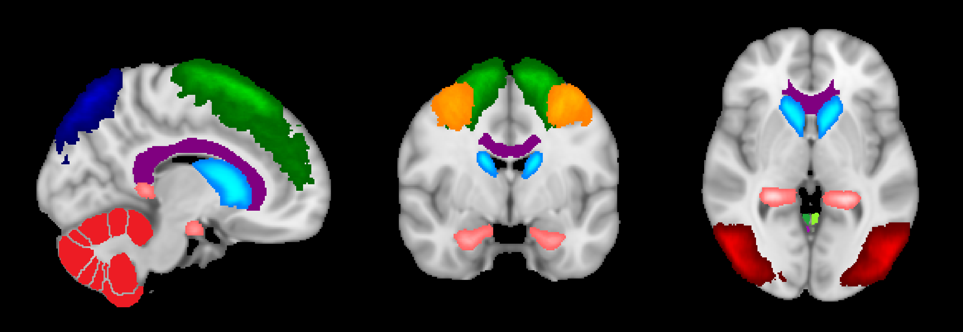
The TSC maps were then registered to their respective T1 anatomicals using FSL’s FLIRT tool8. The anatomicals were then registered to the standard Montreal Neurological Institute (MNI) space, and the saved warping matrix was applied to the respective TSC maps. A combination of the Harvard-Oxford Cortical and Subcortical, JHU tracts, and FSL’s cerebellum atlases were used to segment the TSC maps into grey matter (GM), white matter (WM), cerebrospinal fluid (CSF), hippocampus, cerebellum, occipital lobes, middle frontal gyrus, caudate nucleus, corpus callosum, and superior frontal gyrus regions. Each ROI mask was eroded slightly to account for the broader point spread function (PSF) of the sodium images, and to reduce the chances of partial voluming of ROIs into one another. ANOVA analysis was then performed using MATLAB’s (https://www.mathworks.com/) anovan() function to determine any sources of variance in the regional data – between ROIs, between scans, between subjects, and between methods.
Results
Based on the ANOVA analysis (Figure 1) it was found that there was no significant difference in TSC based on quantitation method (P<0.1085). Furthermore, there was significant difference in repeated scans on the same subjects (P<0.2459). As fully expected, there was variation between the ROIs (P<2.3119x10-218) and subjects (P<7.75x10⁻¹⁰).Conclusions and Discussion
Although this analysis would benefit from more data, especially more subjects, it can be concluded that whichever method is implemented for the quantification of TSC maps, it can be concluded that all three approaches will provide statistically similar results. However, to generalize this conclusion more subjects (both male and female), over at a wide range of ages, is required. Age associated changes in vitreous humor, for example, could lead to difficulties in the generalization of such a method. We are currently assessing contributions to model variance when determining TSC to better determine which approach has the best precision and/or accuracy.Acknowledgements
No acknowledgement found.References
1. Riemer, F., McHugh, D., Zaccagna, F., Lewis, D., McLean, M. A., Graves, M. J., Gilbert, F. J., Parker, G. J. M., & Gallagher, F. A. (2019). Measuring tissue sodium concentration: Cross‐vendor repeatability and reproducibility of 23 Na‐MRI across two sites. Journal of Magnetic Resonance Imaging, 50(4), 1278–1284. https://doi.org/10.1002/jmri.26705
2. Thulborn, K. R. (2018). Quantitative sodium MR imaging: A review of its evolving role in medicine. NeuroImage, 168, 250–268. https://doi.org/10.1016/j.neuroimage.2016.11.056
3. Gerhalter, T., Chen, A. M., Dehkharghani, S., Peralta, R., Adlparvar, F., Babb, J. S., Bushnik, T., Silver, J. M., Im, B. S., Wall, S. P., Brown, R., Baete, S. H., Kirov, I. I., & Madelin, G. (2021). Global decrease in brain sodium concentration after mild traumatic brain injury. Brain Communications, 3(2), fcab051. https://doi.org/10.1093/braincomms/fcab051
4. Coste, A., Boumezbeur, F., Vignaud, A., Madelin, G., Reetz, K., Le Bihan, D., Rabrait-Lerman, C., & Romanzetti, S. (2019). Tissue sodium concentration and sodium T1 mapping of the human brain at 3 T using a Variable Flip Angle method. Magnetic Resonance Imaging, 58, 116–124. https://doi.org/10.1016/j.mri.2019.01.015
5. Stobbe, R., & Beaulieu, C. (2008). Sodium imaging optimization under specific absorption rate constraint. Magnetic Resonance in Medicine, 59(2), 345–355. https://doi.org/10.1002/mrm.21468
6. Sacolick, L. I., Wiesinger, F., Hancu, I., & Vogel, M. W. (2010). B1 mapping by Bloch-Siegert shift. Magnetic Resonance in Medicine, 63(5), 1315–1322. https://doi.org/10.1002/mrm.22357
7. Uecker, M., Ong, F., Tamir, J.I., Bahri, D., Virtue, P., Cheng, J.Y., Zhang, T., & Lustig, M. (2015). Berkeley Advanced Reconstruction Toolbox. Proc Intl Soc Mag Reson Med.
8. Jenkinson, M., Bannister, P., Brady, J. M., & Smith, S. M. (2002). Improved Optimisation for the Robust and Accurate Linear Registration and Motion Correction of Brain Images. NeuroImage, 17(2), 825-841.
Figures