1272

Disentangling the contributions of myelin, neurofilament & microglia to MR contrast: an automated pipeline for voxelwise MR-histology analysis

Daniel Z.L. Kor¹, Saad Jbabdi¹, Jeroen Mollink¹, Istvan N. Huszar¹, Sean Foxley², Menuka Pallebage-Gamarallage³, Connor Scott³, Adele Smart³, Olaf Ansorge³, Karla L. Miller¹, and Amy F.D. Howard¹
¹Wellcome Centre for Integrative Neuroimaging, FMRIB, Nuffield Department of Clinical Neurosciences, University of Oxford, Oxford, United Kingdom, ²Department of Radiology, University of Chicago, Chicago, IL, United States, ³Neuropathology, Nuffield Department of Clinical Neurosciences, University of Oxford, Oxford, United Kingdom

Synopsis

Acquisition of MRI and histology in the same ex-vivo tissue sample enables direct correlation between MR and histologically-derived metrics. Here, we analysed immunohistochemistry images of human visual cortex, anterior cingulate and hippocampus to produce stained area fraction maps for myelin, neurofilaments and microglia. We performed voxelwise correlations between MR parameters (FA, MD, R2*, R1) and histology maps to generally characterise the strength of relationships. We then used partial correlation to identify the unique variance in MR parameters explained by each histological feature, and multiple linear regression to explore how well multiple microstructural properties can together explain MR parameters.

Introduction

Comparison of MRI with histological markers in the same tissue sample provides insight into the cellular correlates of MRI signals, which are notoriously non-specific. Immunohistochemistry (IHC) is a histological technique that uses antibodies to target specific proteins (i.e. proteolipid protein in myelin). One approach uses diaminobenzidine (DAB) to stain the target protein brown, and hematoxylin to counterstain cell bodies purple.

A common semi-quantitative analysis of IHC images uses stained area fraction (SAF), calculated as the number of pixels in a region where the protein-of-interest has been stained by DAB. SAF values can be correlated with MR parameters to investigate hypothesised microstructural sources of MRI.

Here, we have developed a processing pipeline¹ for histology images to automatically extract SAF maps for IHC targeting proteins in myelin, neurofilaments, and microglia. We register² and correlate SAF maps with diffusion-MR (fractional anisotropy, FA; mean diffusivity, MD) and relaxometry (R2*, R1) parameter maps. Using this voxelwise correspondence between IHC and MRI, we explore the relationship between multiple IHC stains and multiple MR parameters. To account for covariance between stains, we use partial correlation to identify the unique variance in MR parameters explained by each targeted protein. We also perform multiple regression with all stains to derive a predictive model of each MR parameter, which may be driven by multiple microstructural features.

Data Acquisition

We acquired MRI and IHC data from several regions of the post-mortem brains of 1 ALS patient and 1 healthy control. All MRI^3,4,5and IHC⁵ protocols have been previously described.

Whole brains were imaged in a 7T whole-body human scanner (Siemens, 1Tx/32Rx head coil) with 3D multi-echo GRE for R2*-mapping³, multi-TI turbo spin-echo for R1-mapping⁵ and diffusion-weighted steady-state free precession for FA- and MD-mapping⁴.

For each brain, 4 tissue slides (6-μm thick) were sectioned from the visual cortex (both hemispheres), anterior cingulate (cingulum bundle, corpus callosum) and hippocampus. Slides were stained for proteins that are surrogate markers for myelin (PLP), neurofilaments (SMI312), microglia (Iba1) and activated microglia (CD68).

Methods

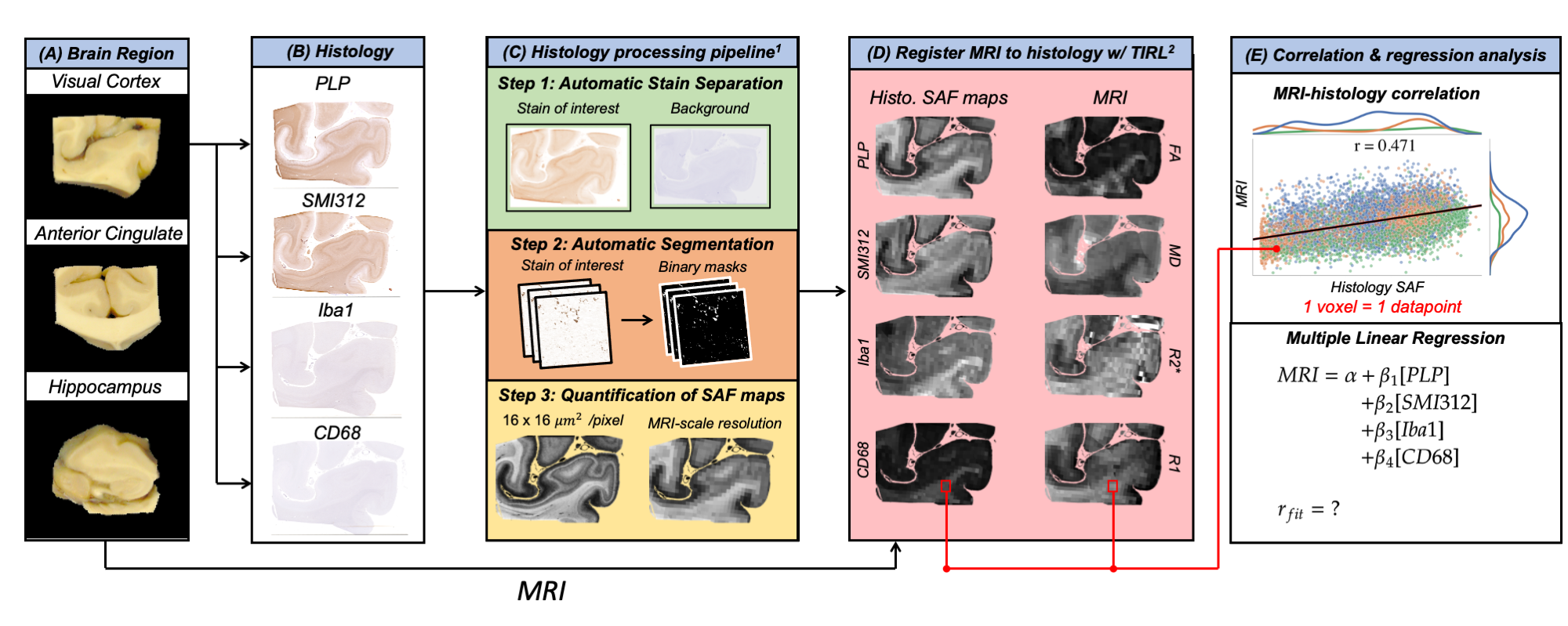
Figure 1 outlines the analysis following data acquisition:

Data Processing (1C): IHC slides were processed via the processing pipeline¹, which utilizes data-driven stain separation and thresholding based on Otsu’s method^6,7 to derive SAF maps. SAF is first calculated in 16-µm² patches.

Data Registration (1D): SAF and MR maps were co-registered to the PLP IHC slides using TIRL², chosen based on PLP’s strong white/grey matter contrast. For each IHC slide, SAF was then calculated within the patch corresponding to each MR voxel, enabling voxelwise MR-IHC correlations.

Correlations and Regression Analysis (1E): For MR-IHC analyses, we pooled voxelwise data across regions and brains. First, we correlated each pairing of MR parameter vs. IHC SAF. Second, we calculated the unique variance of each MR parameter that is explained by an individual stain using partial correlation. Last, we performed multiple regression using all stains together to model a given MR parameter and computed a relative importance measure^8,9 for each stain.

Results and Discussion

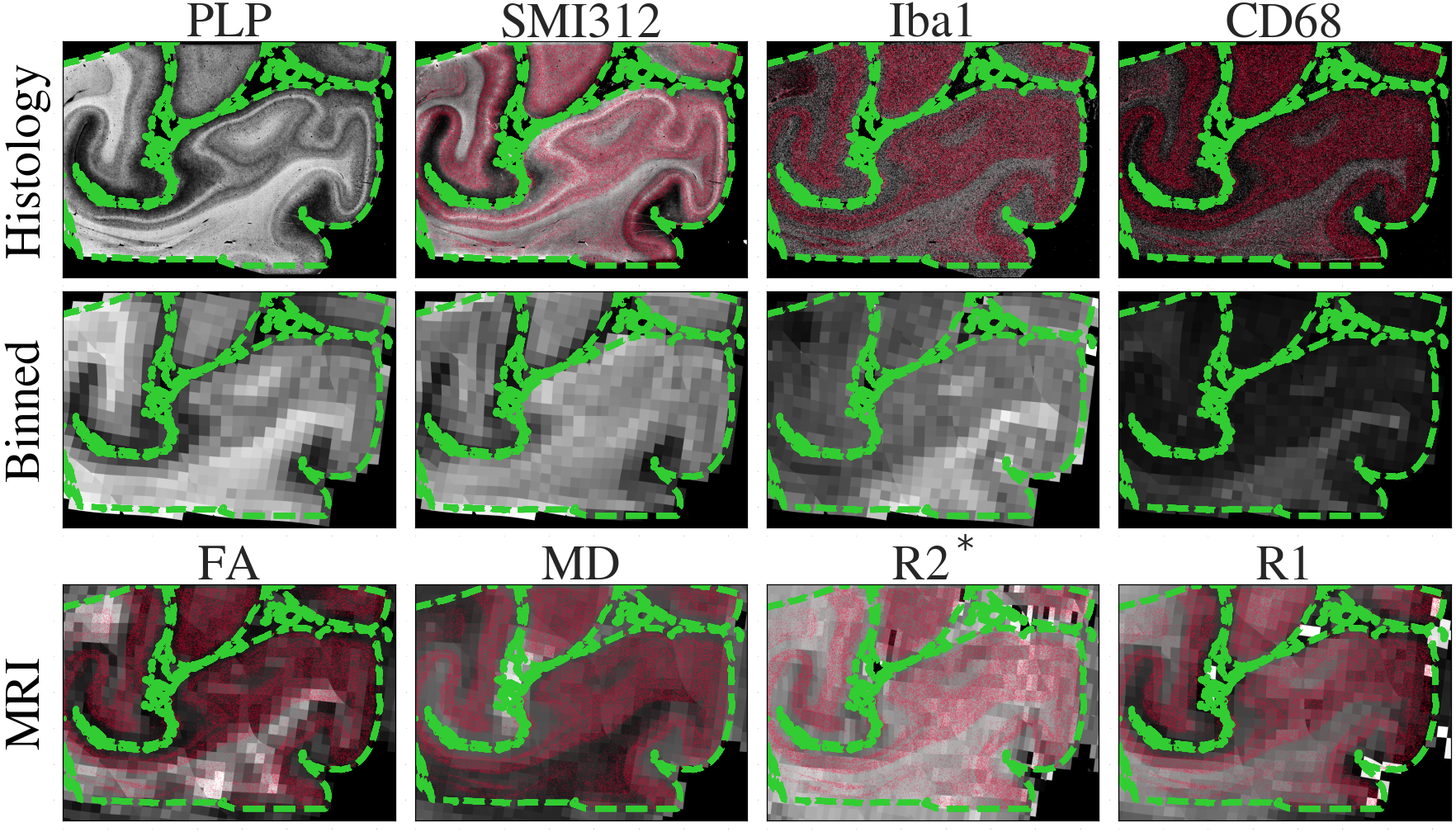
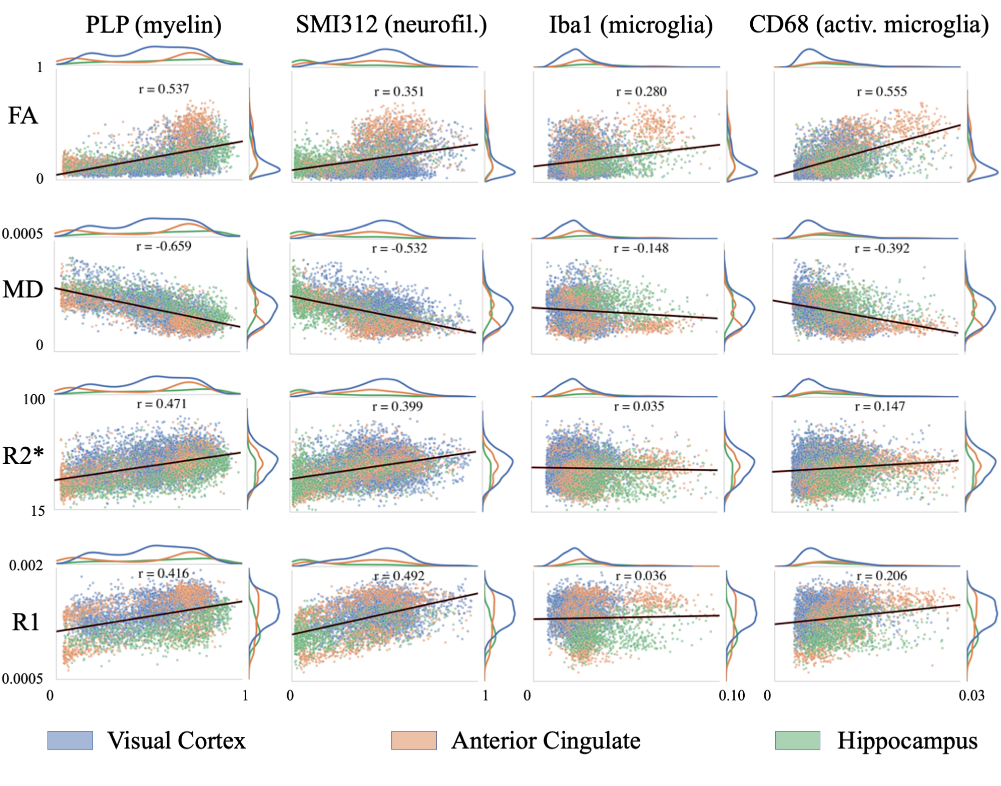
Figure 2 demonstrates the high registration accuracy achieved when co-registering SAF and MR parameter maps via TIRL².

Figure 3 shows pairwise correlations between MR parameters (rows) and stains (columns). The spread in PLP (myelin) and SMI312 (neurofilaments) demonstrates that the chosen brain regions provide good dynamic range. All MR parameters show high correlations with PLP and SMI312 SAF (r=0.35-0.66), though the relationship between FA both PLP and SMI312 appears to be non-linear. Interestingly, CD68 (activated microglia) correlates strongly (r=0.56) with FA.

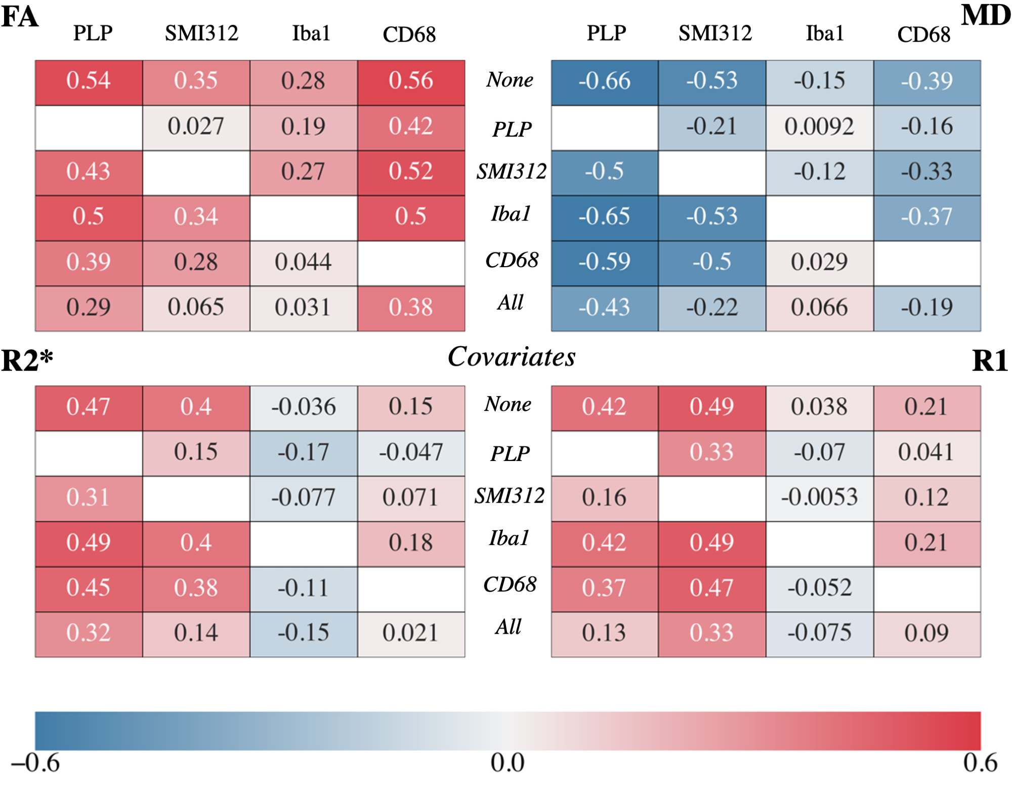
Figure 4 shows the partial correlation coefficients for each MR parameter. In general, these partial correlations emphasize the need to consider multiple potential microstructural causes when validating MR parameters, as highlighted in two notable results.

First, the correlation with SMI312 is greatly reduced after accounting for PLP, though PLP’s correlations remain high (|r| >0.29) in FA, MD and R2* after accounting for SMI312. This suggests that there is unique variance in FA, MD and R2* explained by myelin in particular^10,11, but that associations with neurofilaments may primarily reflect a spatial covariance with myelin rather than a direct relationship. The opposite pattern is seen for R1, suggesting that R1 is sensitive to neurites in general, rather than myelin itself. This is noteworthy since studies report myelin correlating with R1^12,13,14 while not controlling for neurofilaments.

Second, the strikingly high correlation remains between FA and CD68 (r=0.38) after accounting for Iba1 and PLP. The apparent correlation with Iba1 vanishes after accounting for CD68. This points to unique variance in FA being substantially explained by activated microglia, as opposed to all microglia, and suggests FA’s sensitivity to neuroinflammation. Contrarily, FA negatively correlates with neuroinflammation associated with Parkinson’s disease¹⁵ and obesity¹⁶. However, these studies only investigate WM and do not correlate FA with activated microglia, making a direct comparison with our results difficult.

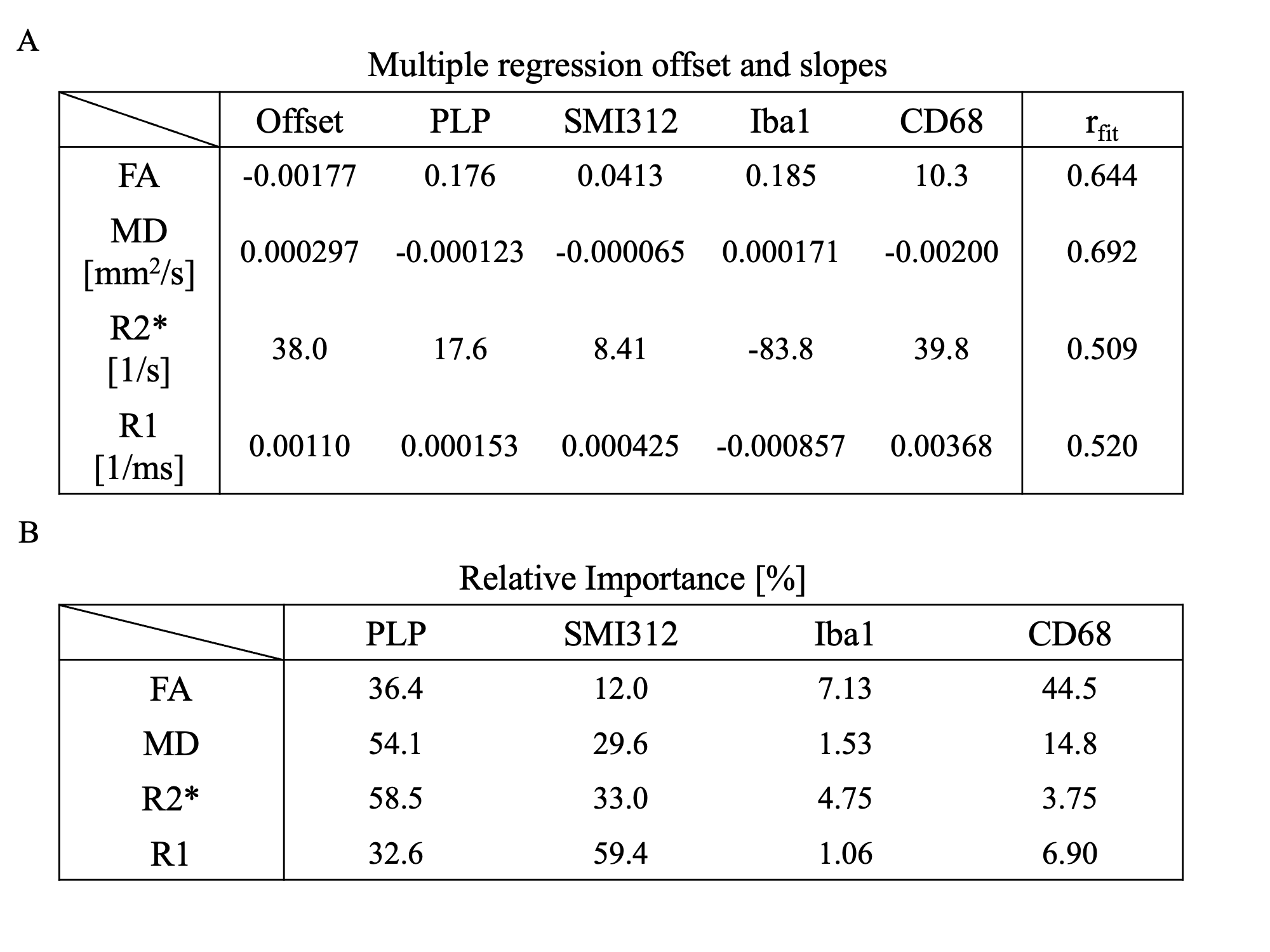
Figure 5A shows how combining multiple stains better explains the variance in each MR parameter. Relative importance (Figure 5B) mirrors partial correlation results, with activated microglia contributing the most to FA (44.5%), neurofilament to R1 (59.4%), and myelin to R2s (58.5%) and MD (54.1%).

Notably, this work does not include other relevant microstructures that affect MRI, such as ferritin^13,14,17. Future work will include other microstructural sources of MR contrast.

Acknowledgements

AFDH and KLM contributed equally to this work. Data acquired was funded by the grant MR/K02213X/1 from the Medical Research Council (MRC). DZLK is supported by the Hrothgar Singaporean Clarendon Scholarship and the Nuffield Department of Clinical Neurosciences studentship. AFDH and INH were supported by the EPSRC and MRC grants (grants EP/L016052/1 and MR/L009013/1). KLM and SJ are supported by the Wellcome Trust (grants WT202788/Z/16/A and WT215573/Z/19/Z). The Wellcome Centre for Integrative Neuroimaging is supported by core funding from the Wellcome Trust (203139/Z/16/Z).

References

1. Kor DZL, Jbabdi S, Mollink J, et al. Automatic extraction of reproducible semi-quantitative histological metrics for MRI-histology correlations. Proceedings of the 29th Annual Meeting of ISMRM. 2021. (abstract 2433)

2. Huszar IN, Pallebage-Gamarallage M, Foxley S, et al. Tensor Image Registration Library: Automated Non-Linear Registration of Sparsely Sampled Histological Specimens to Post-Mortem MRI of the Whole Human Brain.; 2019:849570. doi:10.1101/849570

3. Wang C, Foxley S, Ansorge O, et al. Methods for quantitative susceptibility and R2* mapping in whole post-mortem brains at 7T applied to amyotrophic lateral sclerosis. NeuroImage. 2020;222:117216. doi:10.1016/j.neuroimage.2020.117216

4. Tendler BC, Foxley S, Hernandez-Fernandez M, et al. Use of multi-flip angle measurements to account for transmit inhomogeneity and non-Gaussian diffusion in DW-SSFP. NeuroImage. 2020;220:117113. doi:10.1016/j.neuroimage.2020.117113

5. Pallebage-Gamarallage M, Foxley S, Menke RAL, et al. Dissecting the pathobiology of altered MRI signal in amyotrophic lateral sclerosis: A post mortem whole brain sampling strategy for the integration of ultra-high-field MRI and quantitative neuropathology. BMC Neurosci. 2018;19(1):11. doi:10.1186/s12868-018-0416-1

6. Otsu N. A Threshold Selection Method from Gray-Level Histograms. IEEE Transactions on Systems, Man, and Cybernetics. 1979;9(1):62-66. doi:10.1109/TSMC.1979.4310076

7. Yuan X, Wu L, Peng Q. An improved Otsu method using the weighted object variance for defect detection. Applied Surface Science. 2015;349:472-484. doi:10.1016/j.apsusc.2015.05.033

8. Lindeman RH, Merenda PF, & Gold RZ. Introduction to Bivariate and Multivariate Analysis. 1980. Glenview, IL: Scott, Foresman and Company.

9. Grömping U. Relative Importance for Linear Regression in R: The Package relaimpo. Journal of Statistical Software. 2006;17(1): 1–27.

10. Lazari A, Lipp I. Can MRI measure myelin? Systematic review, qualitative assessment, and meta-analysis of studies validating microstructural imaging with myelin histology. NeuroImage. 2021;230:117744. doi:10.1016/j.neuroimage.2021.117744

11. Mancini M, Karakuzu A, Cohen-Adad J, Cercignani M, Nichols TE, Stikov N. An interactive meta-analysis of MRI biomarkers of myelin. Jbabdi S, Baker CI, Jbabdi S, Does M, eds. eLife. 2020;9:e61523. doi:10.7554/eLife.61523

12. Schmierer K, Scaravilli F, Altmann DR, Barker GJ, Miller DH. Magnetization transfer ratio and myelin in postmortem multiple sclerosis brain. Annals of Neurology. 2004;56(3):407-415. doi:10.1002/ana.20202

13. Stüber C, Morawski M, Schäfer A, et al. Myelin and iron concentration in the human brain: a quantitative study of MRI contrast. Neuroimage. 2014;93 Pt 1:95-106. doi:10.1016/j.neuroimage.2014.02.026

14. Hametner S, Endmayr V, Deistung A, et al. The influence of brain iron and myelin on magnetic susceptibility and effective transverse relaxation - A biochemical and histological validation study. Neuroimage. 2018;179:117-133. doi:10.1016/j.neuroimage.2018.06.007

15. Chiang PL, Chen HL, Lu CH, et al. White matter damage and systemic inflammation in Parkinson’s disease. BMC Neurosci. 2017;18(1):48. doi:10.1186/s12868-017-0367-y

16. Samara A, Murphy T, Strain J, et al. Neuroinflammation and White Matter Alterations in Obesity Assessed by Diffusion Basis Spectrum Imaging. Frontiers in Human Neuroscience. 2020;13:464. doi:10.3389/fnhum.2019.00464

17. Langkammer C, Krebs N, Goessler W, et al. Quantitative MR Imaging of Brain Iron: A Postmortem Validation Study. Radiology. 2010;257(2):455-462. doi:10.1148/radiol.10100495

Figures

Figure 1: An overview of the analysis. A: Brain regions are sectioned for immunohistochemistry (IHC). B: Sections are stained for myelin (PLP), neurofilament (SMI312), all microglia (Iba1) & activated micrgolia (CD68). C: IHC images are processed with a processing pipeline¹ to output stained area fraction (SAF) maps. D: SAF & MRI maps are then co-registered voxel-wise via TIRL². E: Voxels are pooled to perform pairwise correlations and multiple regression between MRI & SAF, where a data point represents a voxel.

Figure 2: Registration evaluation for the visual cortex. Contours of the same tissue mask (green dashed) are overlaid over all co-registered SAF maps (1 pixel here represents SAF calculated in a 16 μm² patch) (first row), SAF maps binned to match MRI data resolution (second row) and MR parameter maps (third row) show good tissue alignment. WM/GM contrast is aligned when overlaying contours of white/grey matter contrast (red) generated from the PLP SAF map. This high registration accuracy enables us to perform voxelwise MR-histology correlations.

Figure 3: Scatterplots used in correlating each MR parameter (rows) and SAF (columns) pair, and their corresponding correlation coefficients, r. The line of best fit (black line) is plotted to visualize trends between each pairing. The visual cortex (blue), anterior cingulate (orange) and hippocampus (green) provide good dynamic range for the MR parameters and SAFs.

Figure 4: Heatmaps of MR partially correlated to different stain’s SAF. For each heatmap, the MR parameter is correlated with each stain’s SAF (columns) while partialling out different stain’s SAF (rows with italicized labels). The first row (“None”) indicates no covariates being partialled out, while the last row (“All”) describes all covariates being partialled out.

Figure 5: Results from the multiple regression of each MR vs. all stains’ SAF. A: As SAF values are unitless, all offsets and slopes are given in units of MR parameters. All show improved fits (r_fit>0.50) relative to single regressions (Figure 1). B: The relative importance^8,9 of a stain’s SAF is the amount of variance it can explain in an MR parameter, averaged over all permutations of multiple regressions that include the specific stain. Values are normalized across stains to get a unit percentage.

Proc. Intl. Soc. Mag. Reson. Med. 30 (2022)

1272

DOI: https://doi.org/10.58530/2022/1272