1264
Robust and efficient R2* estimation in human brain using log-linear weighted least squares
Luke J. Edwards1, Siawoosh Mohammadi1,2, Kerrin J. Pine1, Martina F. Callaghan3, and Nikolaus Weiskopf1,4
1Department of Neurophysics, Max Planck Institute for Human Cognitive and Brain Sciences, Leipzig, Germany, 2Department of Systems Neuroscience, University Medical Center Hamburg-Eppendorf, Hamburg, Germany, 3Wellcome Centre for Human Neuroimaging, UCL Queen Square Institute of Neurology, University College London, London, United Kingdom, 4Felix Bloch Institute for Solid State Physics, Faculty of Physics and Earth Sciences, Leipzig University, Leipzig, Germany
1Department of Neurophysics, Max Planck Institute for Human Cognitive and Brain Sciences, Leipzig, Germany, 2Department of Systems Neuroscience, University Medical Center Hamburg-Eppendorf, Hamburg, Germany, 3Wellcome Centre for Human Neuroimaging, UCL Queen Square Institute of Neurology, University College London, London, United Kingdom, 4Felix Bloch Institute for Solid State Physics, Faculty of Physics and Earth Sciences, Leipzig University, Leipzig, Germany
Synopsis
In vivo maps of R2* in human brain hold promise for neuroscientific investigations. We tested several R2* fitting routines (nonlinear least squares [NLLS; silver standard], auto-regression on linear operations [ARLO], log-linear weighted least square [WLS], and log-linear ordinary least squares [OLS]) for dual flip angle multi-echo FLASH data in simulations and challenging 400 µm resolution in vivo 7T data. Log-linear WLS was found to give a good trade-off between accuracy, precision, and computational time. The method will be available in a future version of the open source hMRI toolbox (hmri.info).
Introduction
In vivo maps of R2* in human brain hold promise for investigations of ageing1, disease2, and cytoarchitecture3.Multiparameter mapping (MPM) efficiently estimates R2* along with R1 and proton density (PD) from dual flip angle (FA; one PD-weighted [PDw] and one T1-weighted [T1w]) multi-echo 3D FLASH data4,5. Log-linear ordinary least squares (OLS), as implemented in the open-source hMRI toolbox (hmri.info)5, is used to robustly estimate R2*, even in the presence of motion artefacts, by assuming a common R2* between the two FAs6.
However, log-linear OLS is non-optimal, as log-transformation induces heteroskedasticity. The optimal log-linear solution requires weighted least squares (WLS), where the weights are proportional to the squared noise-free signals7,8. Iterative approaches improve weight estimation using the last iteration's signal intensities9.
OLS's non-optimality could give rise to spatial R2* precision differences when data quality is spatially varying. An example is whole-brain 7T imaging, where large B0 inhomogeneities10,11 can cause large variation in signal-to-noise-ratio (SNR).
Alternative R2* fitting approaches use the signals directly, rather than log-linearisation. While general nonlinear least squares (NLLS) fitting is slow, auto-regression on linear operations (ARLO) promises similar accuracy in a fraction of the time12. However, for optimal performance ARLO requires knowledge of SNR, which is problematic to routinely obtain.
We evaluated these approaches (OLS, WLS, ARLO, and NLLS) in simulated and 7T in vivo data.
Methods
We modified the hMRI toolbox R2* fitting routine to include NLLS (with OLS initial parameters), ARLO (without debiasing or truncation), and log-linear WLS (WLS1 uses OLS for initial weights9, and WLS3 has three iterations) in addition to the native OLS. The WLS and NLLS implementations parallelise over voxels to reduce runtime.In vivo data were recorded on a Magnetom 7T scanner (Siemens Healthineers, Erlangen). The participant gave written informed consent before scanning. The protocol13 was repeated in two separate sessions; fortuitously in one session the PDw data was strongly corrupted by motion and signal loss, allowing motion, no-motion, and signal loss comparisons. Imaging parameters: 400 µm isotropic resolution, 6 equispaced TEs: [3.3,...,16.3] ms, TR: 31.6 ms, GRAPPA: $$$2\times2$$$, FA(PDw): 5°, FA(T1w): 27°. We used the NLLS result as silver standard for visualisation.
For quantification, (10 mm)3 regions of interest (ROIs) were manually selected in the frontal lobe white matter (WM) based on the PDw volumes6. ROIs were selected based on their homogeneous appearance or because they suffered from signal loss. Because even the homogeneous appearing ROIs still contain some inhomogeneity, R2* maps were smoothed beforehand within a WM mask (Gaussian kernel, σ: 200 µm). Significant differences to the NLLS result were evaluated using two-sample Kolmogorov–Smirnov tests ($$$p < 0.05$$$).
Simulations used in vivo TEs, R2*: 40 s$$$^{-1}$$$, SNR (Rician noise) reflecting a typical in vivo WM voxel, and 105 noise instances. Comparative runtimes were obtained by running 11 simulations and taking the mean time over the last 10; WLS1, WLS3, and NLLS used 8 parallel processors.
Results
Simulations (Fig. 1) showed combining PDw and T1w data improved R2* estimation over just using PDw data for all methods, though the OLS distribution is notably wider than the other distributions. OLS was fastest (0.02 s), then ARLO (0.11 s), WLS1 (0.36 s), WLS3 (0.78 s), and finally NLLS (41.53 s).In vivo R2* maps (Fig. 2) were in line with the simulations, with WLS1 and WLS3 appearing very similar to the NLLS results, whereas OLS showed broad spatial differences, especially in the signal loss region.
Quantitative comparisons (Fig. 3) supported the visual assessment: the OLS R2* distribution significantly differed from NLLS in all cases (asterisk in Fig. 3), whereas WLS1 R2* did not significantly differ in any of the cases. WLS3 and ARLO R2* distributions were each significantly different from the NLLS distribution in at least one case. OLS was particularly affected in the signal loss region, though all methods showed bias in this case compared to the other cases, probably due to noise-floor effects.
Discussion
WLS1 results were consistent with NLLS but approximately $$$100\times$$$ faster to compute. In contrast, OLS was fastest, but showed large differences to NLLS in all cases.ARLO improved on OLS, and took less time than WLS1, but still showed relatively large differences to NLLS. This relatively poor performance could be because we did not perform debiasing and truncation based on SNR12, which is challenging to estimate reliably.
In terms of motion-robustness, all methods improved upon OLS, itself already relatively motion robust6.
The lack of improvement in vivo of iterative WLS3 over WLS1 may well reflect inaccuracy in our NLSS silver standard, or that no fixed point exists for outlier voxels (e.g. in Fig. 2, blood vessels are more prominent in the WLS3 differences).
Maximum likelihood/a posteriori methods14,15 could improve accuracy and (at the expense of precision) account for Rician noise bias16, but are in general very slow.
Conclusion
Log-linear WLS estimation of a common R2* across multi-flip angle multi-echo data offers a good trade-off between accuracy, precision, and computational time in challenging data. The method will be available in a future version of the hMRI toolbox (hmri.info).Acknowledgements
The research leading to these results has received funding from the European Research Council under the European Union's Seventh Framework Programme (FP7/2007-2013) / ERC grant agreement n° 616905. SM was funded by the German Research Foundation (DFG Priority Program 425 2041 “Computational Connectomics,” (MO 2397/5-1), DFG Emmy Noether Stipend: MO 2397/4-1).The Max Planck Institute for Human Cognitive and Brain Sciences and Wellcome Centre for Human Neuroimaging have institutional research agreements with Siemens Healthcare. NW holds a patent on acquisition of MRI data during spoiler gradients (US 10,401,453 B2). NW was a speaker at an event organized by Siemens Healthcare and was reimbursed for the travel expenses.References
1. Callaghan, M.F., Freund, P., Draganski, B., Anderson. E., Cappelletti, M., Chowdhury, R., Diedrichsen, J., FitzGerald, T.H.B., Smittenaar, P., Helms, G., Lutti, A., and Weiskopf, N. "Widespread age-related differences in the human brain microstructure revealed by quantitative magnetic resonance imaging", Neurobiol. Aging, 35.8:1862-1872 (2014). https://doi.org/10.1016/j.neurobiolaging.2014.02.0082. Zhao, Y., Raichle, M.E., Wen, J., Benzinger, T.L., Fagan, A.M., Hassenstab, J., Vlassenko, A.G., Luo, J., Cairns, N.J., Christensen, J.J., Morris, J.C., and Yablonskiy, D.A., "In vivo detection of microstructural correlates of brain pathology in preclinical and early Alzheimer Disease with magnetic resonance imaging", Neuroimage, 148:296-304 (2017). https://doi.org/10.1016/j.neuroimage.2016.12.026
3. McColgan, P., Helbling, S., Vaculčiaková, L., Pine, K., Wagstyl, K., Attar, F. M., Edwards, L., Papoutsi, M., Wei, Y., Van den Heuvel, M.P., Tabrizi, S.J., Rees, G., and Weiskopf, N., "Relating quantitative 7T MRI across cortical depths to cytoarchitectonics, gene expression and connectomics", Hum. Brain Mapp., 42.15:4996-5009 (2021). https://doi.org/10.1002/hbm.25595
4. Weiskopf, N., Suckling, J., Williams, G., Correia, M., Inkster, B., Tait, R., Ooi, C., Bullmore, E., and Lutti, A.. "Quantitative multi-parameter mapping of R1, PD*, MT, and R2* at 3T: a multi-center validation", Front. Neurosci., 7:95 (2013). https://doi.org/10.3389/fnins.2013.00095
5. Tabelow, K., Balteau, B., Ashburner, J., Callaghan, M.F., Draganski, B., Helms, G., Kherif, F., Leutritz, T., Lutti, A., Phillips, C., Reimer, E., Ruthotto, L., Seif, M., Weiskopf, N., Ziegler, G., and Mohammadi, S., "hMRI – A toolbox for quantitative MRI in neuroscience and clinical research", Neuroimage, 194:191-210 (2019). https://doi.org/10.1016/j.neuroimage.2019.01.029
6. Weiskopf, N., Callaghan, M.F., Josephs, O., Lutti A., and Mohammadi S., "Estimating the apparent transverse relaxation time (R2*) from images with different contrasts (ESTATICS) reduces motion artifacts", Front. Neurosci., 8:278 (2014). https://doi.org/10.3389/fnins.2014.00278
7. MacFall, J.R., Riederer, S.J. and Wang, H.Z., "An analysis of noise propagation in computed T2, pseudodensity, and synthetic spin-echo images", Med. Phys., 13:285-292 (1986). https://doi.org/10.1118/1.595956
8. Salvador, R., Peña, A., Menon, D.K., Carpenter, T.A., Pickard, J.D. and Bullmore, E.T., "Formal characterization and extension of the linearized diffusion tensor model", Hum. Brain Mapp., 24:144-155 (2005). https://doi.org/10.1002/hbm.20076
9. Veraart, J., Sijbers, J., Sunaert, S., Leemans, A., and Jeurissen, B., "Weighted linear least squares estimation of diffusion MRI parameters: Strengths, limitations, and pitfalls", Neuroimage, 81:335-346 (2013). https://doi.org/10.1016/j.neuroimage.2013.05.028
10. Van de Moortele, P.-F., Pfeuffer, J., Glover, G.H., Ugurbil, K. and Hu, X., "Respiration-induced B0 fluctuations and their spatial distribution in the human brain at 7 Tesla", Magn. Reson. Med., 47:888-895 (2002). https://doi.org/10.1002/mrm.10145
11. Stockmann, J.P., and Wald, L.W., "In vivo B0 field shimming methods for MRI at 7 T", Neuroimage, 168:71-87 (2018). https://doi.org/10.1016/j.neuroimage.2017.06.013
12. Pei, M., Nguyen, T.D., Thimmappa, N.D., Salustri, C., Dong, F., Cooper, M.A., Li, J., Prince, M.R. and Wang, Y., "Algorithm for fast monoexponential fitting based on Auto-Regression on Linear Operations (ARLO) of data", Magn. Reson. Med., 73:843-850 (2015). https://doi.org/10.1002/mrm.25137 Erratum: 17.
13. Trampel, R., Bazin, P.-L., Pine, K., and Weiskopf, N., "In-vivo magnetic resonance imaging (MRI) of laminae in the human cortex", Neuroimage, 197:707-715 (2019). https://doi.org/10.1016/j.neuroimage.2017.09.037
14. Bonny, J.-M., Zanca, M., Boire, J.-Y. and Veyre, A., "T2 maximum likelihood estimation from multiple spin-echo magnitude images", Magn. Reson. Med., 36:287-293 (1996). https://doi.org/10.1002/mrm.1910360216
15. Balbastre, Y., Brudfors, M., Azzarito, M., Lambert, C., Callaghan, M.F., and Ashburner, J. "Joint Total Variation ESTATICS for Robust Multi-parameter Mapping". In: Martel, A.L. et al. (eds), MICCAI 2020. LNCS, 12262:53-63. Springer (2020). https://doi.org/10.1007/978-3-030-59713-9_6
16. Andersson, J.L.R., "Maximum a posteriori estimation of diffusion tensor parameters using a Rician noise model: Why, how and but", Neuroimage, 42.4:1340-1356 (2008). https://doi.org/10.1016/j.neuroimage.2008.05.053
17. Pei, M., Nguyen, T.D., Thimmappa, N.D., Salustri, C., Dong, F., Cooper, M.A., Li, J., Prince, M.R. and Wang, Y., "Erratum to: Algorithm for fast monoexponential fitting based on Auto-Regression on Linear Operations (ARLO) of data (Magn Reson Med 2015;73:843-850)", Magn. Reson. Med., 82:1576-1576 (2019). https://doi.org/10.1002/mrm.27807
Figures
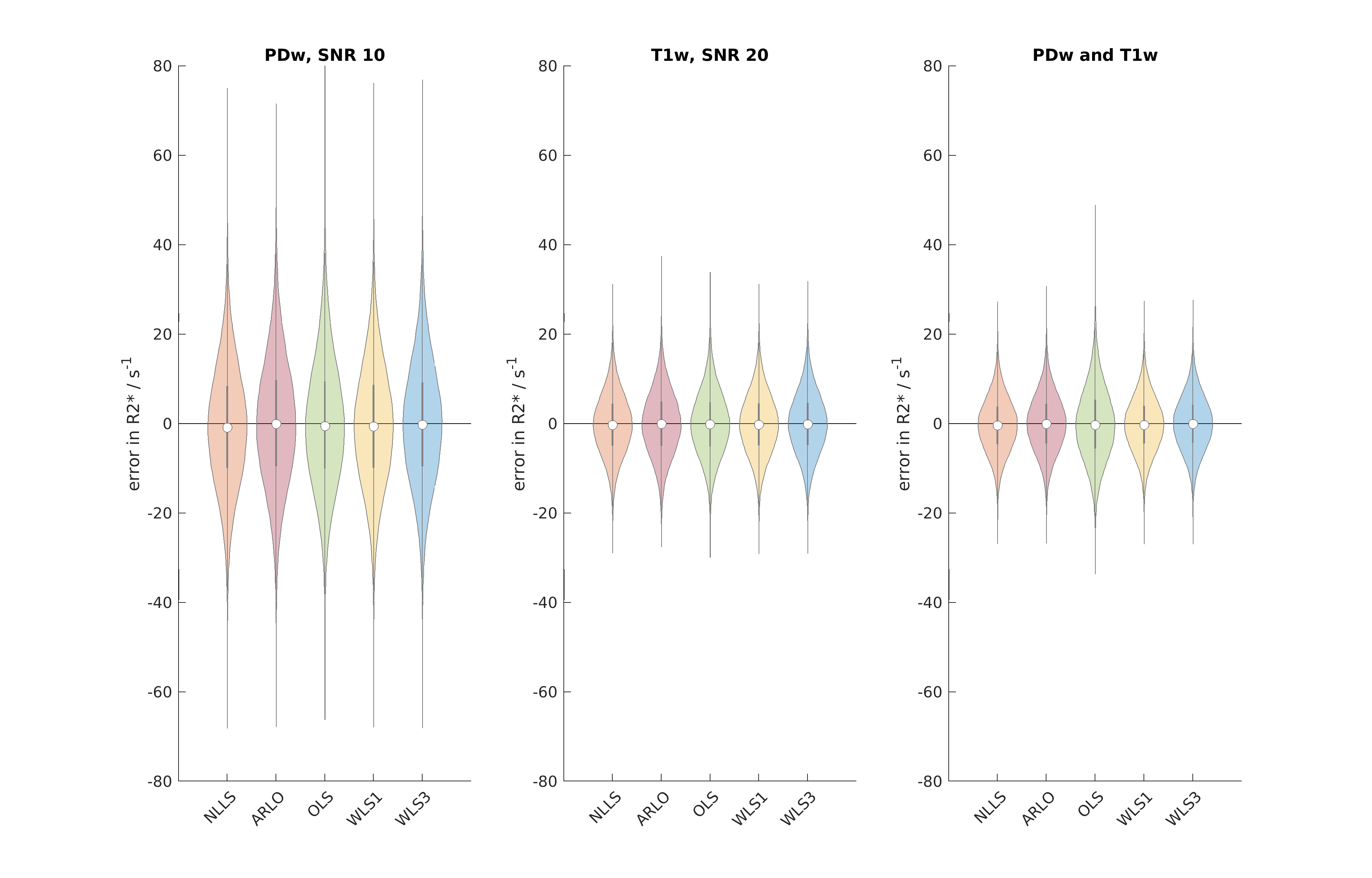
Fig. 1: Violin plots of simulation results for a typical voxel using the 7T protocol. The dot shows the median, the grey vertical bar the interquartile range, and the shaded area the density. SNR values for PDw and T1w data were based on estimates from the in vivo data.
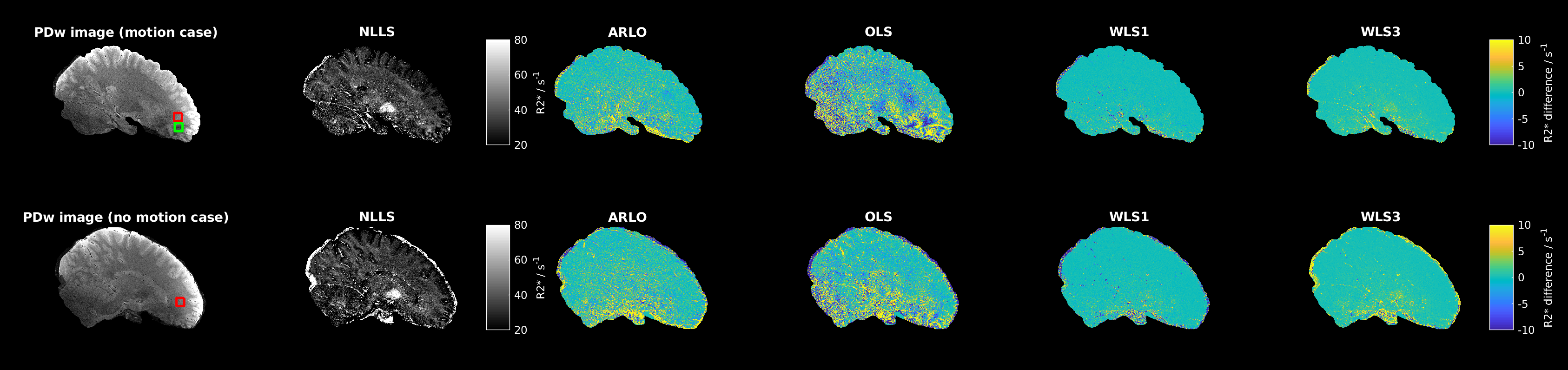
Fig. 2: R2* maps computed with each method. Top row: data with motion artefacts. Bottom row: data without clear motion artifacts. Left column: PDw images (TE 8.5 ms) showing ROIs used in Fig. 3. Red boxes: homogeneous ROI. Green box: ROI with signal loss. Second column: R2* map estimated with NLLS. Other columns: difference between NLLS R2* and other R2* estimates.
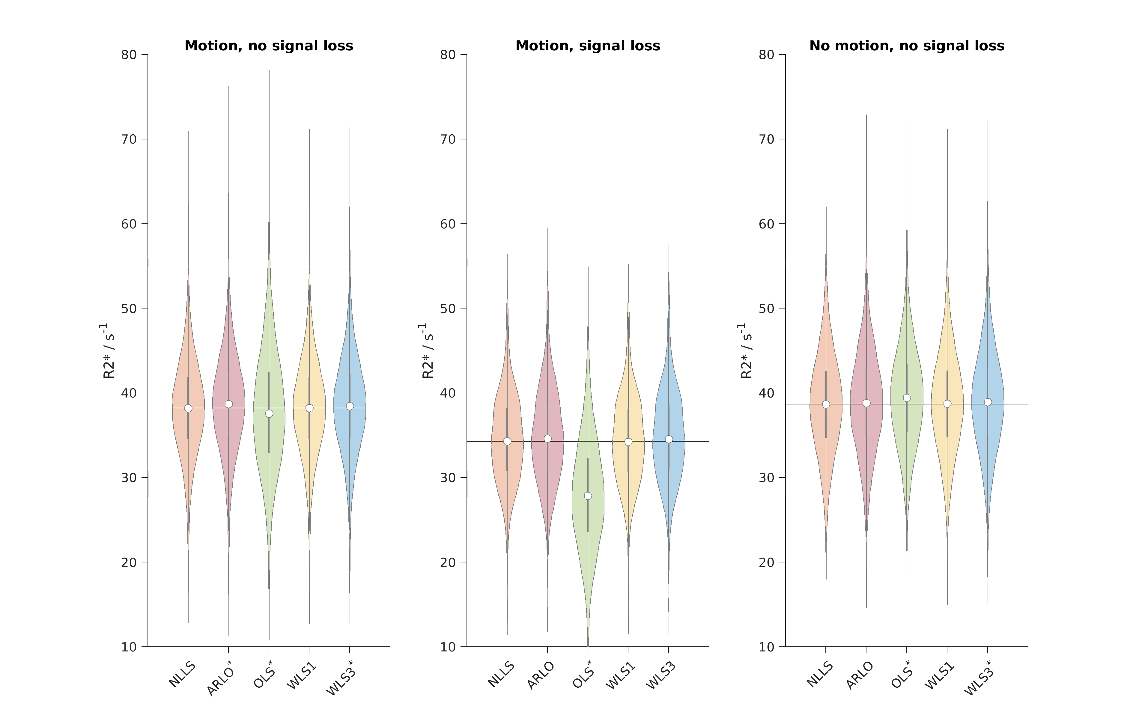
Fig. 3: Violin plots of R2* distributions in WM RoIs. The dot shows the median, the grey vertical bar the interquartile range, the shaded area the density, and the black line the median NLLS R2*. Motion/no motion case: homogeneous ROI (red box in Fig. 2; motion: left; no motion: right). Motion case: additional ROI strongly affected by signal loss (green box in Fig. 2; middle). Voxels outside the WM mask were excluded. *: significant difference to the NLLS result.
DOI: https://doi.org/10.58530/2022/1264