INTRODUCTION

Framewise co-activity patterns of functional MRI (fMRI) data may reflect the transient synchronization and coordination across brain regions ^[1-4]. For instance, with high-intensity frames of resting state fMRI (rsfMRI) time series, Liu and Duyn identified granulated co-activation patterns (CAPs) that resembled the resting state brain networks ^[4]. Yet, it remains unknown whether the opposite side, i.e., the low intensities or negative values (NegVal) of a normalized rsfMRI time series, carry such information. In response, the present study trained variational autoencoder (VAE) models ^[5] using both positive values (PosVal) and NegVals of normalized rsfMRI data and evaluated the two models on a separate dataset.

METHODS

Datasets and preprocessing. Two rsfMRI sessions from HCP ^[6] (rfMRI_REST1_LR or R1LR, and rfMRI_REST2_LR or R2LR) were included. R1LR was used to train the two VAE models, and R2LR was used as a separate dataset for evaluation.

For both sessions, the time series of each voxel was z-scored and thresholded with the 85th and 15th percentiles of the entire time series, respectively, resulting in a PosVal and a NegVal transient CAPs at each frame. These maps were then down sampled to 1cm isotropic. The NegVals were flipped and both datasets were normalized to [0,1] before training.

VAE setting and training. Two VAE models ^[2,5] were trained on the PosVal and NegVal datasets of R1LR. They had the same structure, with 2222 hidden variables and 15 latent variables. To prevent overfitting, dropout layers were added after the ReLU activation layers of both models. For both datasets, subjects were randomly divided into the training (N=768) and validation group (N=256) with a 7:3 ratio. To reduce noise, volumes with fewer than 30 remaining voxels after thresholding were dropped.

Comparison of model parameters. Weight parameters were plotted as matrices for qualitative comparison. To compare the learned latent variables, we generated an image for the unit latent vector along each latent dimension using the corresponding decoder. The resultant images from the two models were matched so that the mutual information between each pair was maximized.

Comparison of model performance. The trained models were used to reconstruct the transient patterns in the new PosVal and NegVal datasets of R2LR. The reconstruction losses from both models were calculated for each subject, and they were statistically compared using the paired student-t test.

RESULTS

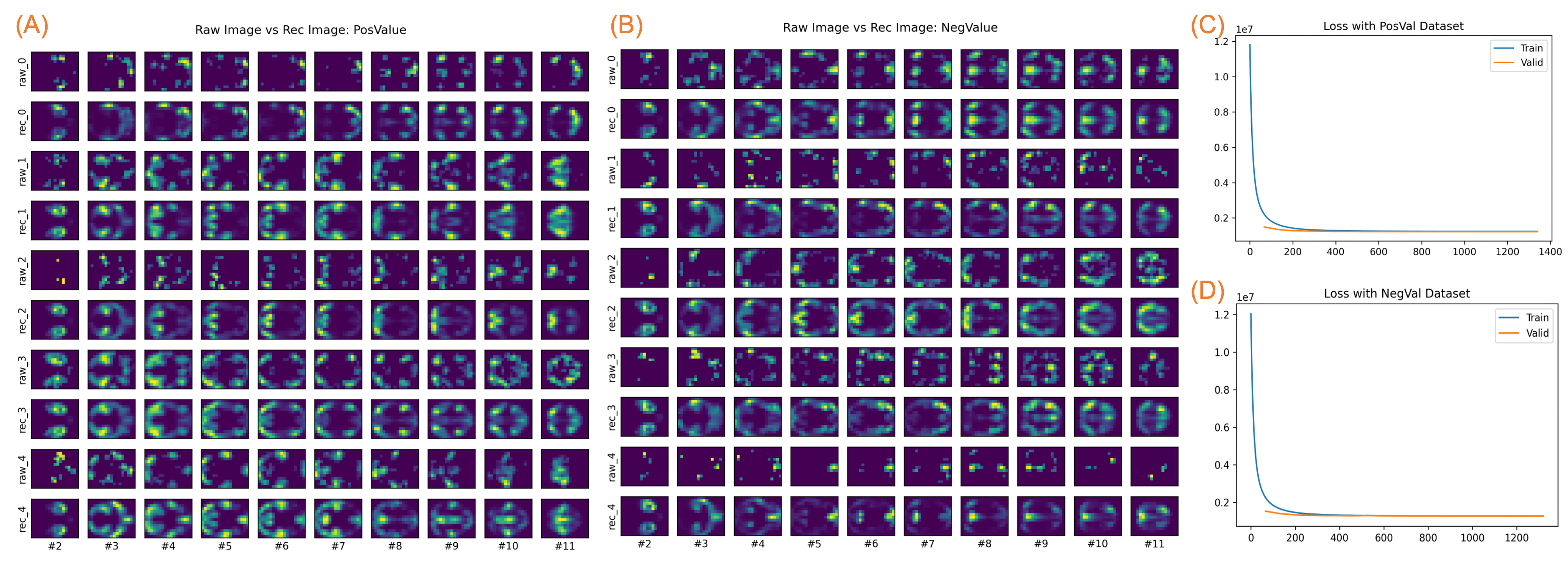
Model training on R1LR. Figure 1 shows the model training on the PosVal and NegVal datasets of R1LR. As seen in the panels A and B, both PosVal and NegVal datasets demonstrated meaningful activity patterns that resembled the resting state brain networks, indicating the low-intensity or NegVal frame carry meaningful information as the high-intensity or PosVal ones do.

The VAE models worked well for both datasets. The loss curves for both trainings converged, as shown in the panels C and D. With the trained models, images were reconstructed with a high similarity with the raw images, as illustrated in the five random samples in the panels A and B.

Note that the reconstructed images were generally smoother than the raw images. The latter might miss some parts of a brain region due to the hard thresholding in the preprocessing step.

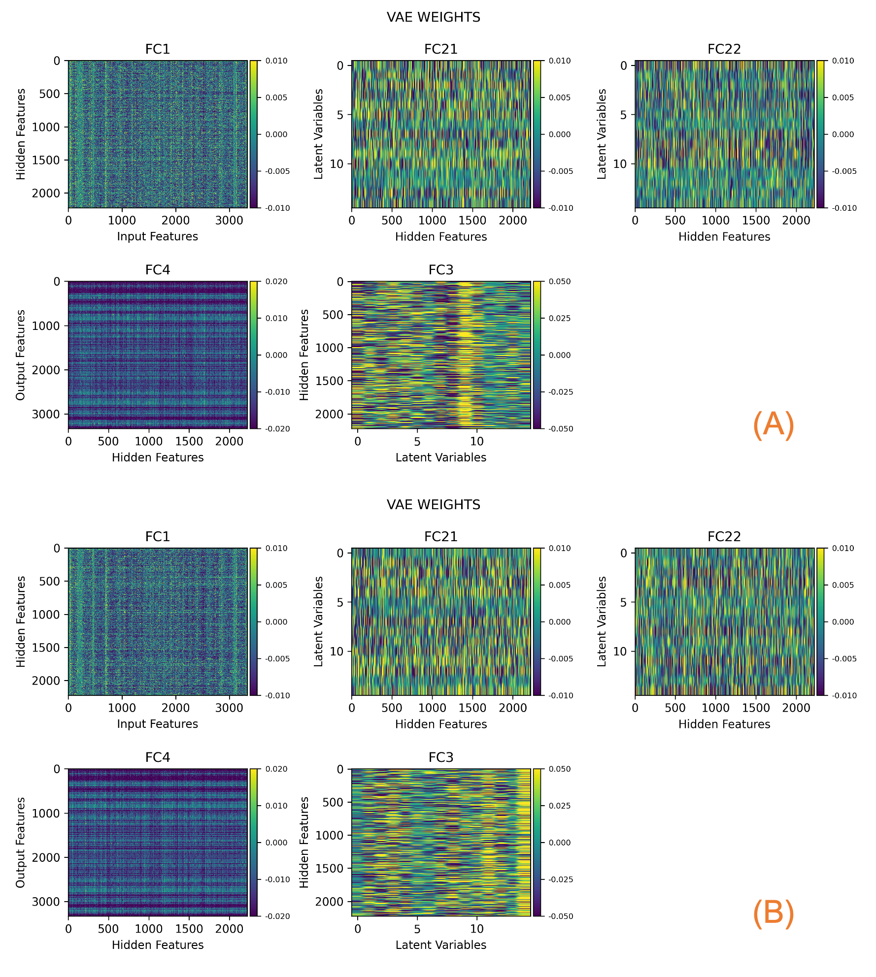
Model parameters and latent representation. The models obtained with PosVal and NegVal datasets were similar. Figure 2 depicts the model parameters for the PosVal dataset (A) and the NegVal dataset (B). The similar texture in FC1 and in FC4 suggests similar mapping between image features and hidden features. FC21, FC22, and FC were not directly compared due to lack of correspondence.

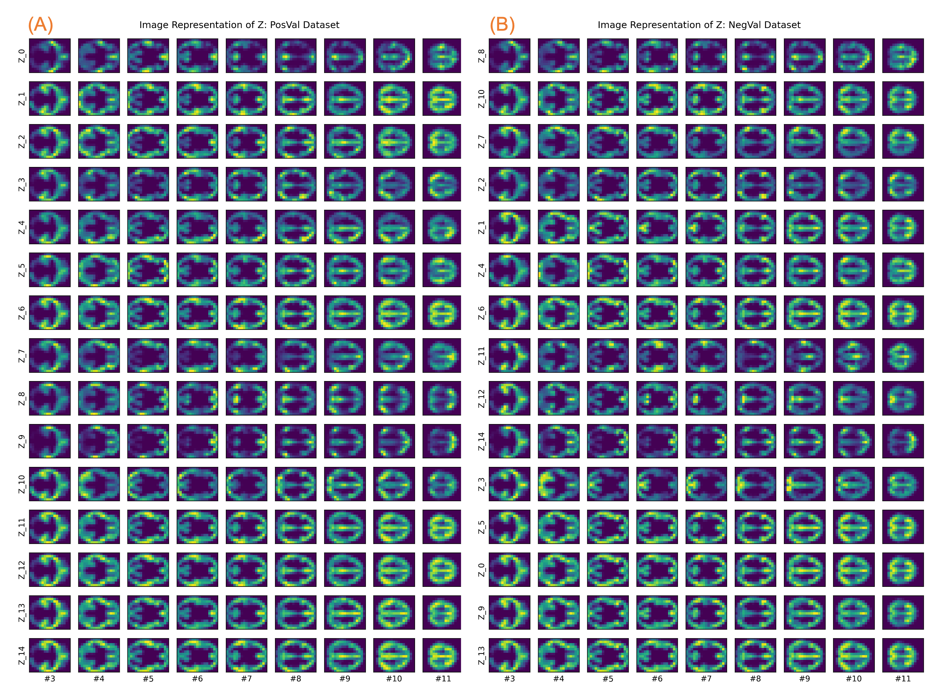
Model similarity also existed in the image representation of latent variables. Figure 3 demonstrated the images constructed with the unit latent variables from the PosVal dataset (A) and the NegVal dataset (B), respectively. As seen, the images resembled resting state brain networks or part of them. Importantly, the high similarity between images in A and B suggests the underlying latent variables may represent the same transient co-activity pattern.

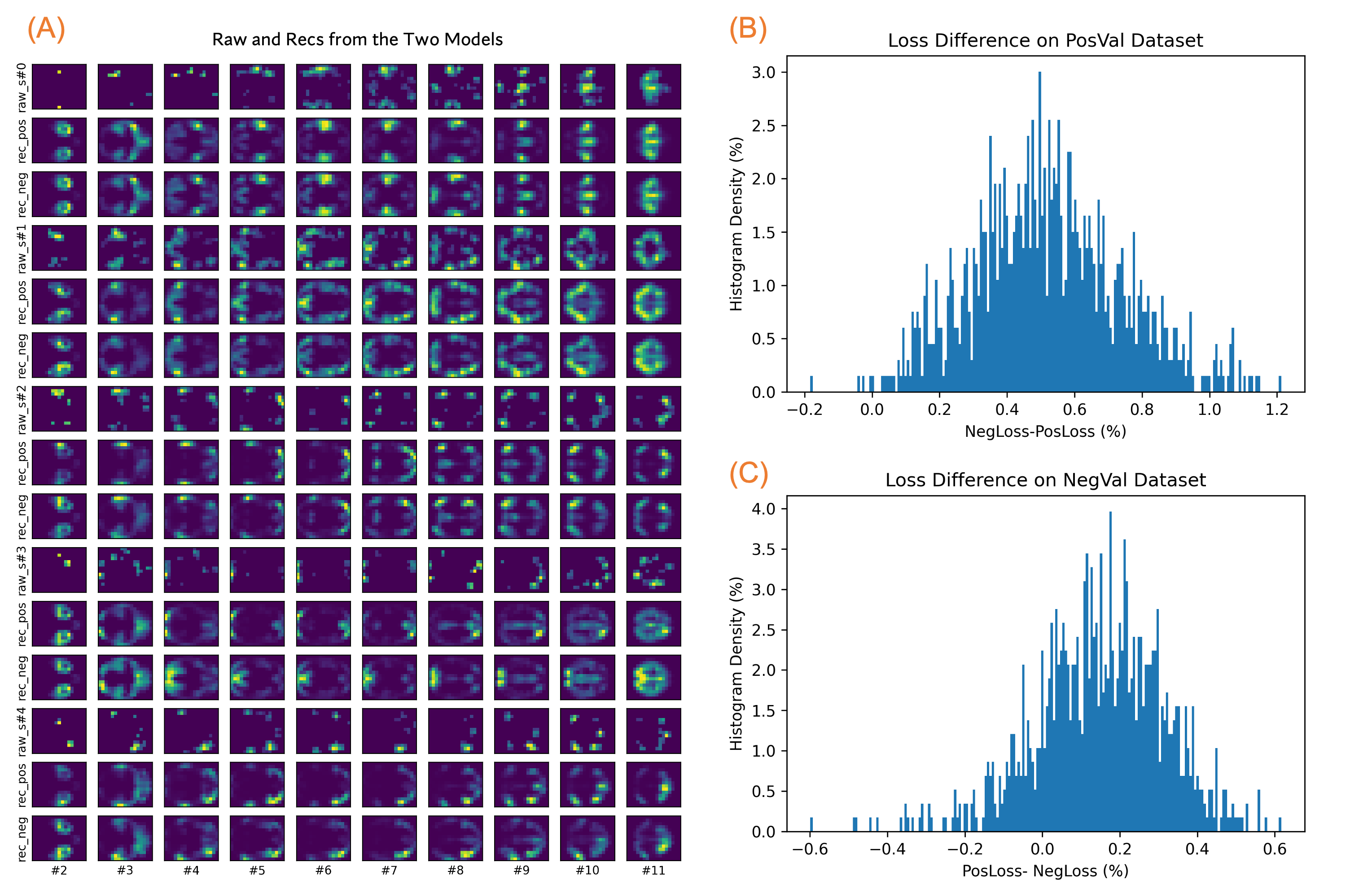
Model performance. The obtained models from R1LR were used to reconstruct images in the new PosVal and NegVal datasets of R2LR. Figure 4A illustrates four random samples of raw images and reconstrued images with the two models. It seems the learned models can accurately reconstruct images in the new datasets.

The model differences in reconstruction losses are depicted in the panels B and C, respectively. For the PosVal dataset of R2LR, the PosVal model had a superior performance compared to the NegVal model, and vice versa (p<10^-4). However, the performance gain ( mean: 0.52%, stdev: 0.22 for the PosVal model on the PosVal dataset; mean: 0.15%, stdev: 0.17 for the NegVal model on the NegVal dataset) was rather small, indicating that either model may work well on either dataset.

DISCUSSION & CONCLUSION

The present study trained and compared variational autoencoder models using positive values and negative values of normalized rsfMRI data. We found the two models were very similar, suggesting that the negative-value frames reflect similar transient brain synchronization patterns as the positive-value ones do. These negative-value time frames can provide additional training samples for neural network models on framewise brain dynamic analysis.

Acknowledgements

No acknowledgement found.