1171

Flip-angle map calculation via keyhole reconstruction in uniform and variable-density 2D-spiral hyperpolarized ¹²⁹Xe MRI

Joseph W Plummer^1,2, Abdullah S Bdaiwi^1,2, Mariah L Costa^1,2, Matthew M Willmering¹, Zackary I Cleveland^1,2,3, and Laura L Walkup^1,2,3,4
¹Center for Pulmonary Imaging Research, Department of Pulmonary Medicine, Cincinnati Children's Hospital Medical Center, Cincinnati, OH, United States, ²Biomedical Engineering, University of Cincinnati, Cincinnati, OH, United States, ³Department of Radiology, Cincinnati Children's Hospital Medical Center, Cincinnati, OH, United States, ⁴Department of Pediatrics, Cincinnati Children's Hospital Medical Center, Cincinnati, OH, United States

Synopsis

Hyperpolarized ¹²⁹Xe-MRI is prone to B₁-inhomogeneity-induced signal artifacts, that often obscure pulmonary abnormalities. B₁-inhomeogeneity can be corrected by calculating a flip-angle map and rescaling the images. Current methods to acquire a flip-angle map in 2D-spiral sequences require two-successive images to be collected in a single breath-hold, doubling scan duration. We demonstrate that flip-angle maps can be calculated from a single image acquisition using keyhole reconstruction. Furthermore, analytical methods can be used to minimize the amount of required oversampling. This approach enables accurate B₁-artifact correction, with minimal impact to scan-duration, making it especially useful for short breath-hold studies.

Introduction

Hyperpolarized ¹²⁹Xe-MRI is a powerful imaging technique, most-well known for its ability to characterize regional gas-uptake and airway-obstruction in the lungs from a single breath-hold image^1-3. Its feasibility is particularly benefitted by center-out sequences, such as 2D-spiral, where sampling-efficiency and scan-duration, and thus breath-hold duration, are improved. However, ¹²⁹Xe-MRI is highly sensitive to regional differences in applied flip-angle caused by B₁-field inhomogeneity. This may cause signal artifacts that obscure pulmonary abnormalities, including ventilation deficits, and therefore require correction.

An accurate means to correct for B₁-variations is to measure a flip-angle map, and retrospectively rescale the acquired image. When acquisition-time is much less than the in-vivo T₁ (~20s)⁴, flip-angle maps can be generated by acquiring two images within the same breath-hold, and calculating signal decay between them⁵. While this ‘paired-image’ approach produces accurate flip-angle maps, it doubles the scan-duration – increasing the length and difficulty of the breath-hold maneuver. Here, we propose using keyhole-reconstruction combined with either uniform or variable-density 2D-spiral sequences to generate the two images from a single-image acquisition^6,7.

Theory

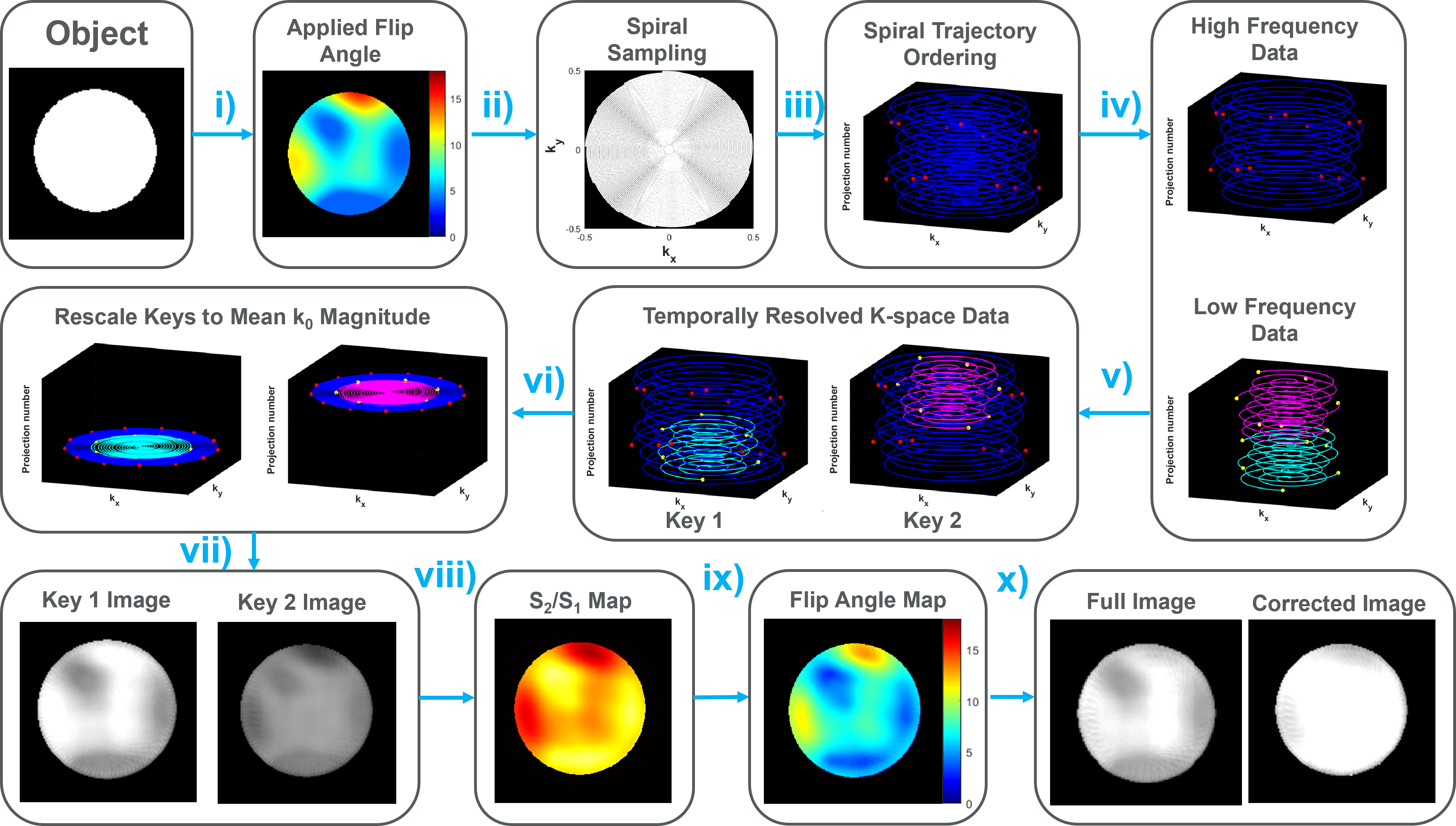
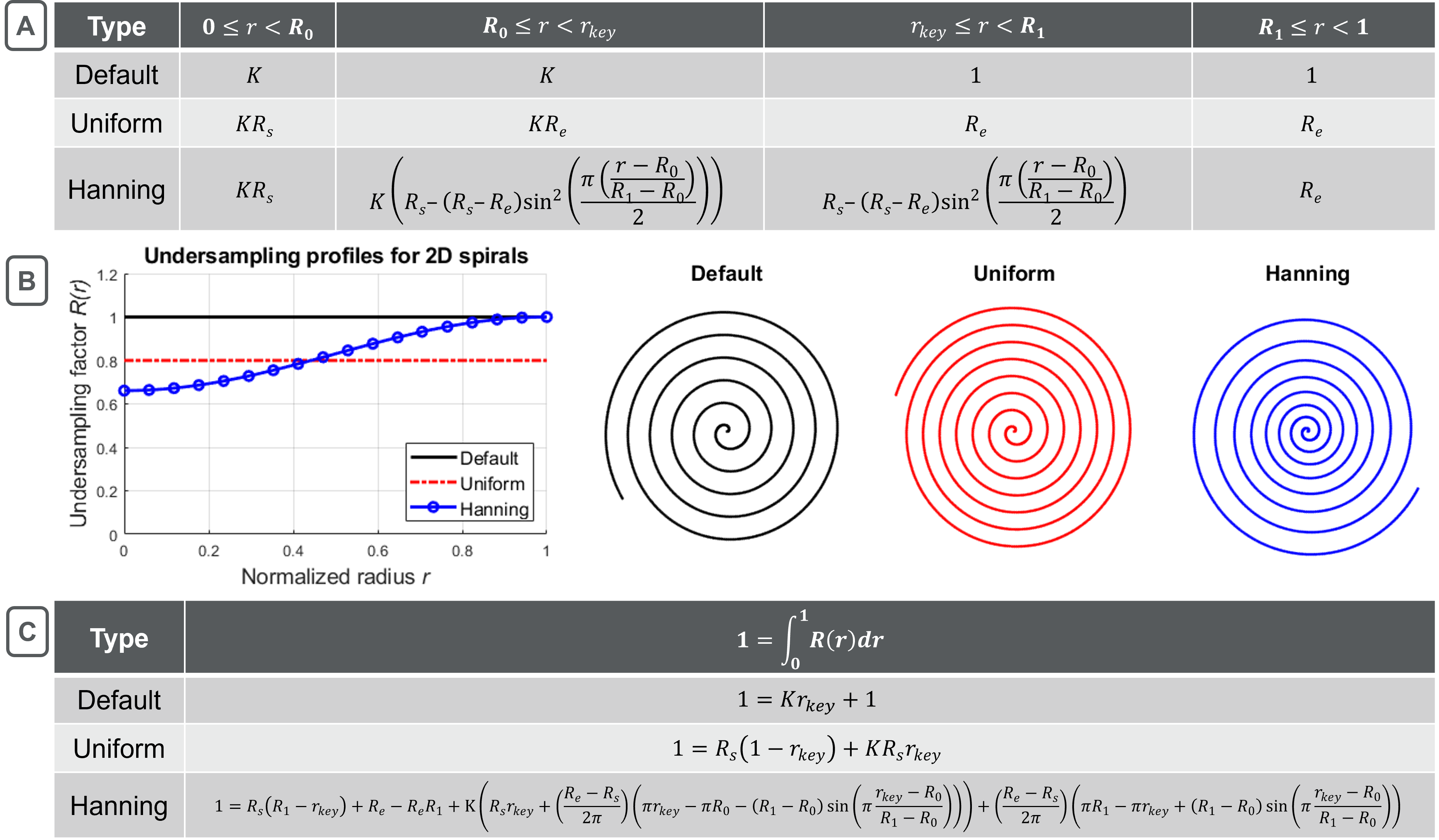
In keyhole-reconstruction, dynamic low-frequency k-space data is divided into K ‘keys’ and combined with the high-frequency k-space data (‘keyhole’) to generate K key-images (K=2 for this work). Voxel-by-voxel signal decay between key-images can be used to calculate a flip-angle map (Fig. 1). The level of spatial detail that can be resolved in the flip-angle map is controlled by the key-radius, r_key. To prevent aliasing artifacts that arise from Nyquist-undersampling inside the key, the 2D-spiral sequence must be oversampled. The degree of oversampling depends on the shape, direction, and sampling-density of the trajectories, and the post-processing details: r_key, and K. A general equation for the degree of oversampling required is given by:
$$1 = \int_{0}^{1} R(r) \,dr, \tag{1}$$
where R(r) is the undersample factor of an Archimedean spiral at normalized radial-position, r, from the center of k-space. A fully-sampled spiral sequence has R=1, an oversampled uniform spiral sequence has R<1, and a variable-density spiral sequence has non-constant R(r) (Fig. 2(A,B)). The division of low-frequency k-space into K keys means that R(r) can be represented as piecewise function from the center of k-space, to r_key, to the edge of k-space. Once a sufficient r_key is chosen, Eq. 1 can be solved to determine the required oversampling profile (Fig. 2(C)).

Methods

Simulations were performed in MATLAB (Mathworks, Natick, MA), using a digital-phantom with a spatially varying applied flip-angle (Figs. 1&2). Matrix=200², spiral-interleaves=100, K=2, r_key=0.1-0.9, R=0.9, uniform-density spiral-out. Calculated flip-angle maps were compared against the applied map using the voxel root-mean square-difference, μ_diff^₂, and the variance difference, σ_diff^₂.

Imaging was performed on a Philips-Achieva 3T scanner, with hyperpolarized-¹²⁹Xe (25-35% polarization⁸, via Polarean 9820A, Durham, NC). Scans were performed on ¹²⁹Xe-gas phantoms (1-L Tedlar bag) and in-vivo (healthy male, 30years and cystic-fibrosis female, 21years), under protocol approved by our local Institutional Review Board (with FDA IND-123,577). Imaging parameters: Field-of-view (FOV)=(350-400)x(350-400)x200mm³, resolution=3x3x15mm³, acquisition-time=5ms, echo-time=1.52ms, repetition-time=11.0ms, spiral-interleaves=13-29, flip-angles=9-18⁰. Images were reconstructed using open-source non-cartesian software⁹.

Results

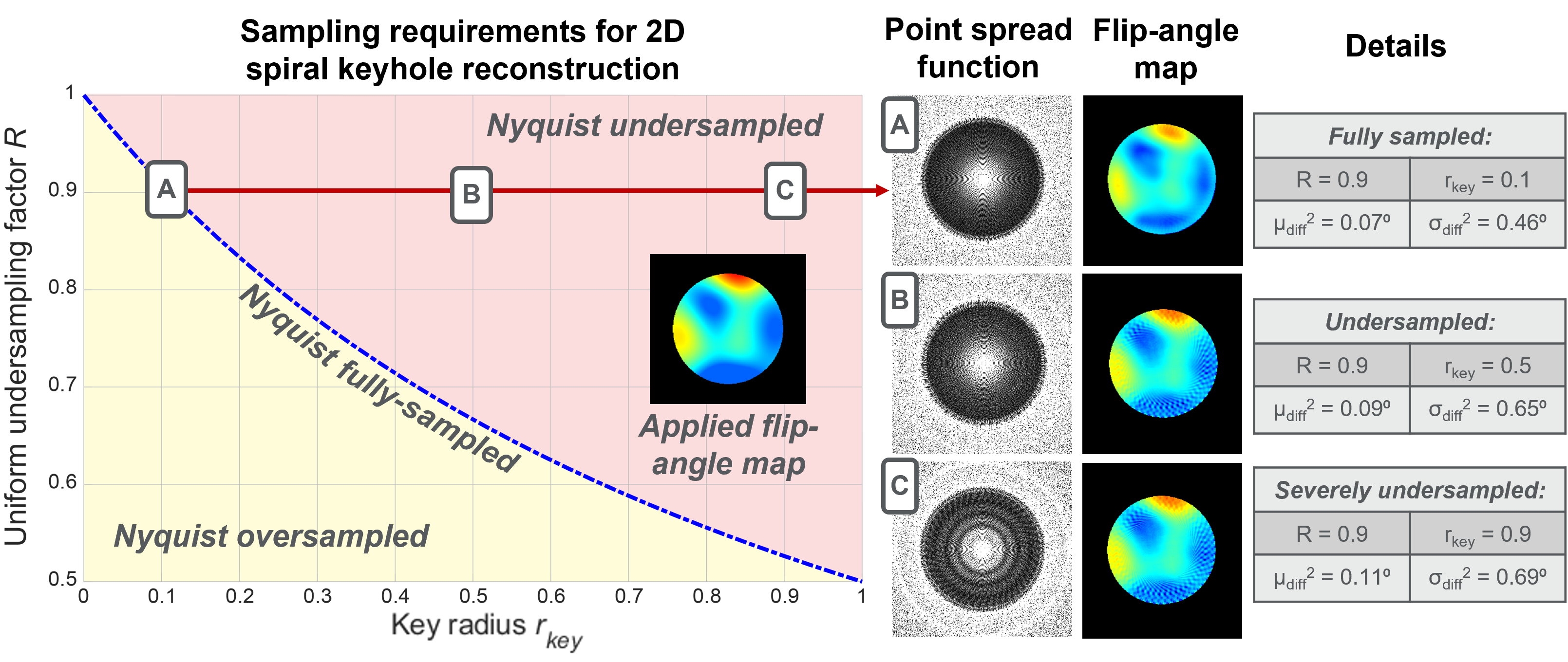
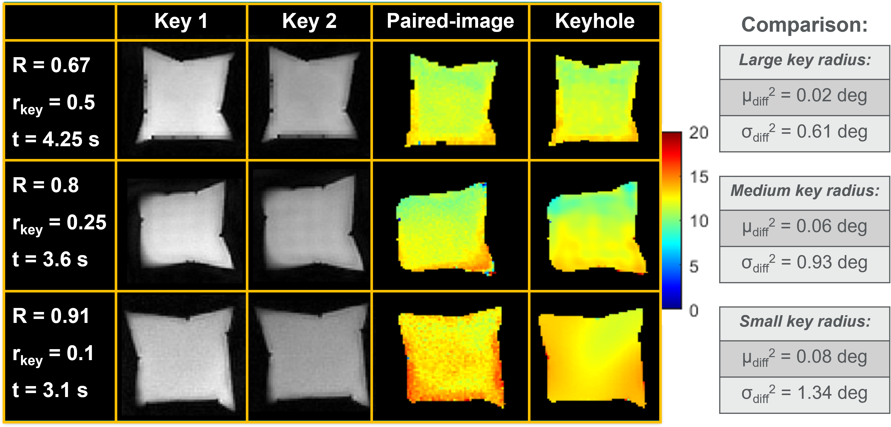
Nyquist-undersampling effects that occur by not meeting Eq. 1 are shown using simulations in Fig. 3. Alias-free flip-angle map reconstructions were achieved using r_key=0.1, with R=0.9 applied uniform-oversampling (μ_diff^₂=0.07⁰, σ_diff^₂=0.46⁰) (Fig. 3(A)). Figs. 3(B,C) show reconstructions for the same R, but r_key=0.5 and r_key=0.9. Here, aliasing artifacts are generated within the supported-FOV of the point-spread-functions, and the accuracy of the flip-angle maps decreased, respectively: μ_diff²=0.09⁰, σ_diff²=0.65⁰, and μ_diff²=0.11⁰, σ_diff²=0.69⁰.

The effects of reconstructing with various r_key are shown in Fig. 4. Optimal flip-angle maps were obtained using the largest r_key: r_key=0.5, R=0.67, at a scan-duration of t=4.25s (μ_diff²=0.02⁰, σ_diff²=0.61⁰ against the paired-image flip-angle map). Shorter scan-durations were possible with r_key=0.25, R=0.8, t=3.6s and r_key=0.1, R=0.91, t=3.1s; however, these flip-angle maps were less accurate (μ_diff²=0.06⁰, σ_diff²=0.93⁰, and μ_diff²=0.08⁰, σ_diff²=1.34⁰, respectively).

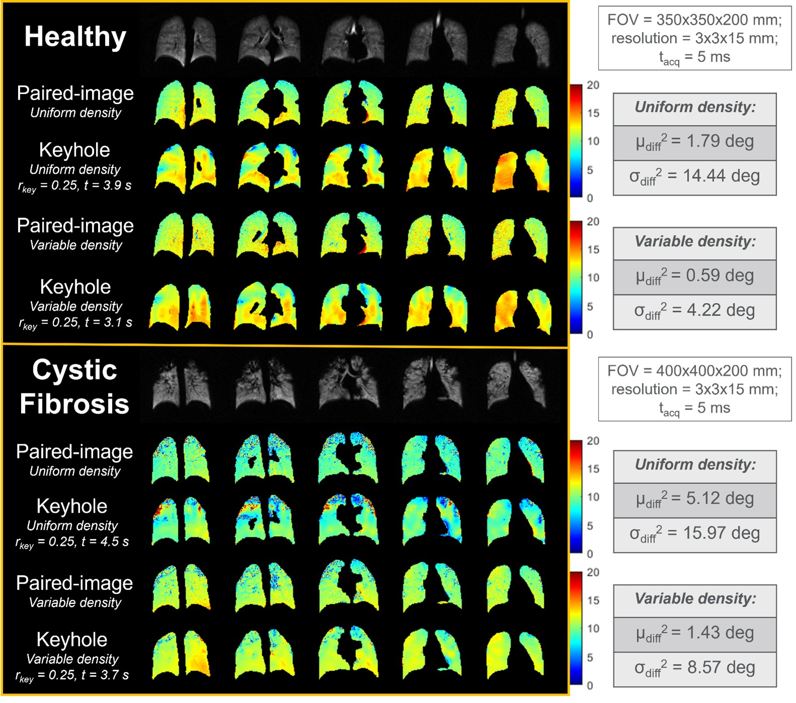
Uniform and variable-density (via Hanning-window) 2D-spiral images were collected in-vivo to test keyhole-reconstruction (Fig. 5). Comparisons between the keyhole and paired-image generated flip-angle maps gave: healthy uniform: μ_diff²=1.79⁰, σ_diff²=14.44⁰; variable-density: μ_diff²=0.59⁰, σ_diff²=4.22⁰; cystic-fibrosis uniform: μ_diff²=5.12⁰, σ_diff²=15.97⁰; variable-density: μ_diff²=1.43⁰, σ_diff²=8.57⁰. Variable-density spirals had ~3-fold greater accuracy and ~20% shorter scan-durations than uniform spirals.

Discussion

In general, keyhole-reconstructions produced spatially similar flip-angle maps to the paired-image approach. Notably, reconstructions with a larger key-radius delivered greater accuracy. However, these required a greater degree of initial oversampling to prevent Nyquist-undersampling artifacts from propagating into the flip-angle map. In turn, this increased the scan-duration. To minimize scan-duration and prevent map artifacts, the key-radius must be balanced with the amount of initial oversampling.

Accuracy and scan-duration was enhanced by using variable-density spirals, with increased density at center. This was more efficient for keyhole-reconstruction, as only the central k-space information needed oversampling to avoid aliasing in the key-images. Consequently, scan-durations were shortened by >20%, and accuracy was improved ~3-fold, when compared to uniform-density spirals.

Conclusion

Keyhole-reconstruction can be used to calculate accurate flip-angle maps from a single 2D-spiral image-acquisition. Such maps are generated with minimal impact to scan-duration and can be optimized further for various sequence parameters. This is especially useful in ¹²⁹Xe-MRI studies where short scan-durations are necessary, such as for children and patients with compromised respiratory-function. This work can be used to apply corrections for B₁-inhomogeneity, with minimal impact to scan-duration.

Acknowledgements

The authors would like to thank Dustin J. Basler for polarizing ¹²⁹Xe for this study. Additionally, we would like to thank the following sources for research funding and support: R01HL131012 and R01HL143011.

References

1. Walkup, L.L. and J.C. Woods, Translational applications of hyperpolarized ³He and ¹²⁹Xe. NMR Biomedicine, 2014. 27(12): p. 1429-38.

2. Bdaiwi, A.S., et al., Improving hyperpolarized ¹²⁹Xe ADC mapping in pediatric and adult lungs with uncertainty propagation. NMR Biomedicine, 2021: p. e4639.

3. Niedbalski, P.J., et al., Protocols for multi-site trials using hyperpolarized ¹²⁹Xe MRI for imaging of ventilation, alveolar-airspace size, and gas exchange: A position paper from the ¹²⁹Xe MRI clinical trials consortium. Magnetic Resonance in Medicine, 2021. 86(6): p. 2966-2986.

4. Mugler, J.P. and T.A. Altes, Hyperpolarized ¹²⁹Xe MRI of the human lung. Journal Magnetic Resonance Imaging, 2013. 37(2): p. 313-31.

5. Miller, G.W., et al., Hyperpolarized ³He lung ventilation imaging with B1-inhomogeneity correction in a single breath-hold scan. Magma, 2004. 16(5): p. 218-26.

6. Niedbalski, P.J. and Z.I. Cleveland, Improved preclinical hyperpolarized ¹²⁹Xe ventilation imaging with constant flip angle 3D radial golden means acquisition and keyhole reconstruction. NMR Biomedicine, 2021. 34(3): p. e4464.

7. Niedbalski, P.J., et al., Mapping and correcting hyperpolarized magnetization decay with radial keyhole imaging. Magnetic Resonance Medicine, 2019. 82(1): p. 367-376.

8. Plummer, J.W., et al., A semi-empirical model to optimize continuous-flow hyperpolarized ¹²⁹Xe production under practical cryogenic-accumulation conditions. Journal of Magnetic Resonance, 2020. 320: p. 106845.

9. Robertson, S.H., et al., Optimizing 3D non-cartesian gridding reconstruction for hyperpolarized ¹²⁹Xe MRI—focus on preclinical applications. Concepts in Magnetic Resonance Part A, 2015. 44(4): p. 190-202.

Figures

Workflow for keyhole-reconstruction of a 2D-spiral sampled digital phantom, with a simulated applied flip-angle map. (i) Apply spatially-varying flip-angle with (ii) multiple RF-excitations, (iii) visualized as a stack. (iv) Separate high/low-frequency data into key/keyhole. (v) Divide key-data into two keys, and recombine with keyhole. (vi) Normalize data to mean k₀ for each key. (vii) Reconstruct key-images, and (viii) divide. (ix) Calculate flip-angle map via⁷. (x) Correct image^5,7.

Example implementations of variable-density 2D-spiral trajectories: default, uniform, and hanning-window. (A) Table containing piecewise functions describing how the undersample-factor, R(r), varies when ranging k-space radius from r=0 to r=1. K=number of keys, R_s and R_e = start and end undersample factor, R₀ and R₁ = start and end variable-density function locations, respectively. (B) Visual representations of (A). (C) Solutions to Eq. 1 for the three spirals used in this example. r_key can be solved for in terms of K, R_s, R_e, R₀, and R₁.

Diagram showing the effects of reconstructing with various r_key for a given uniform undersample factor. (Left) Graph of Eq. 1, with undersampled (red) and oversampled (yellow) regions. (Middle) Point spread functions for three simulations [A,B,C] based on Fig. 2. (Right) Details for measured vs applied flip-angle maps and summary of the root-mean square-difference, μ_diff², and the variance-difference, σ_diff², of the voxels.

(Left) Table containing single slices of hyperpolarized-¹²⁹Xe phantom (1-L Tedlar bag) scanned with various r_key, and a fully sampled R according to Eq. 1. Column 1) independent variables and scan duration, t; columns 2-3) key-images (single slice); column 4) paired-image flip-angle map according to⁵; column 5) keyhole flip-angle map. (Right) Comparisons between paired and keyhole methods (root-mean square-difference, μ_diff², and the variance difference, σ_diff², of the voxels).

(Left) In-vivo (healthy and cystic fibrosis) flip-angle maps. Comparisons are made between uniform and variable-density (Hanning) spiral sampling, which delivers similar results with reduced scan duration. The applied R(r) is fully-sampled for r_key=0.25, according to Eq. 1. (Right) Comparisons between paired and keyhole methods (root-mean square-difference, μ_diff², and the variance difference, σ_diff², of the voxels).

Proc. Intl. Soc. Mag. Reson. Med. 30 (2022)

1171

DOI: https://doi.org/10.58530/2022/1171