Introduction

Graph Signal Processing (GSP) has seen increased use in the field of neuroimaging ¹. The ability to derive information not just from time series at distinct locations but also from structural or functional connections between them, has been shown to be powerful. GSP is performed using graphs; signals structured as a combination of nodes and edges, both of which represent data. The nodes corresponding to points in the volume and edges to their connection, be it structural or functional ². Despite flourishing in brain imaging, literature applying GSP to musculoskeletal imaging is sparse. We looked to perform an investigation into possible applications of GSP to musculoskeletal imaging, more specifically muscle BOLD (mBOLD) ^2,3 of the lower leg (Gastrocnemius, Soleus, and Tibialis Anterior). We investigated GSPs using both the windowed coherence and Higuchi Fractal Dimension approaches ^5,6, between nodes as functional connections.

Methods

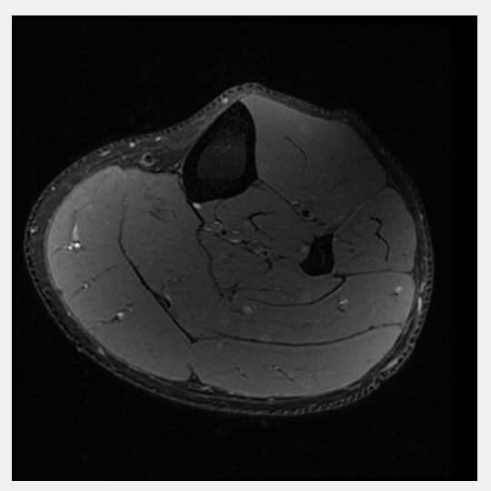
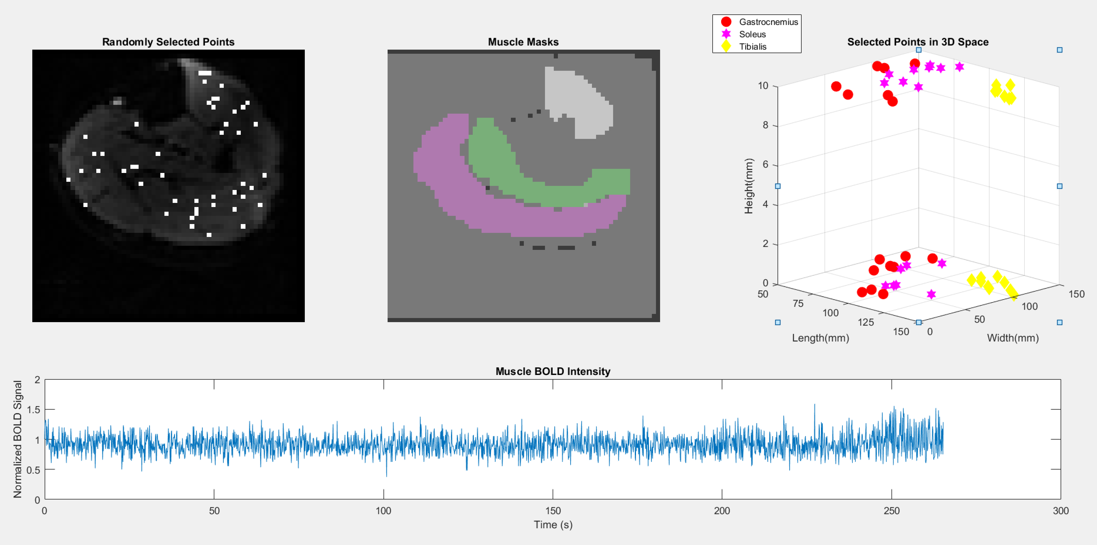
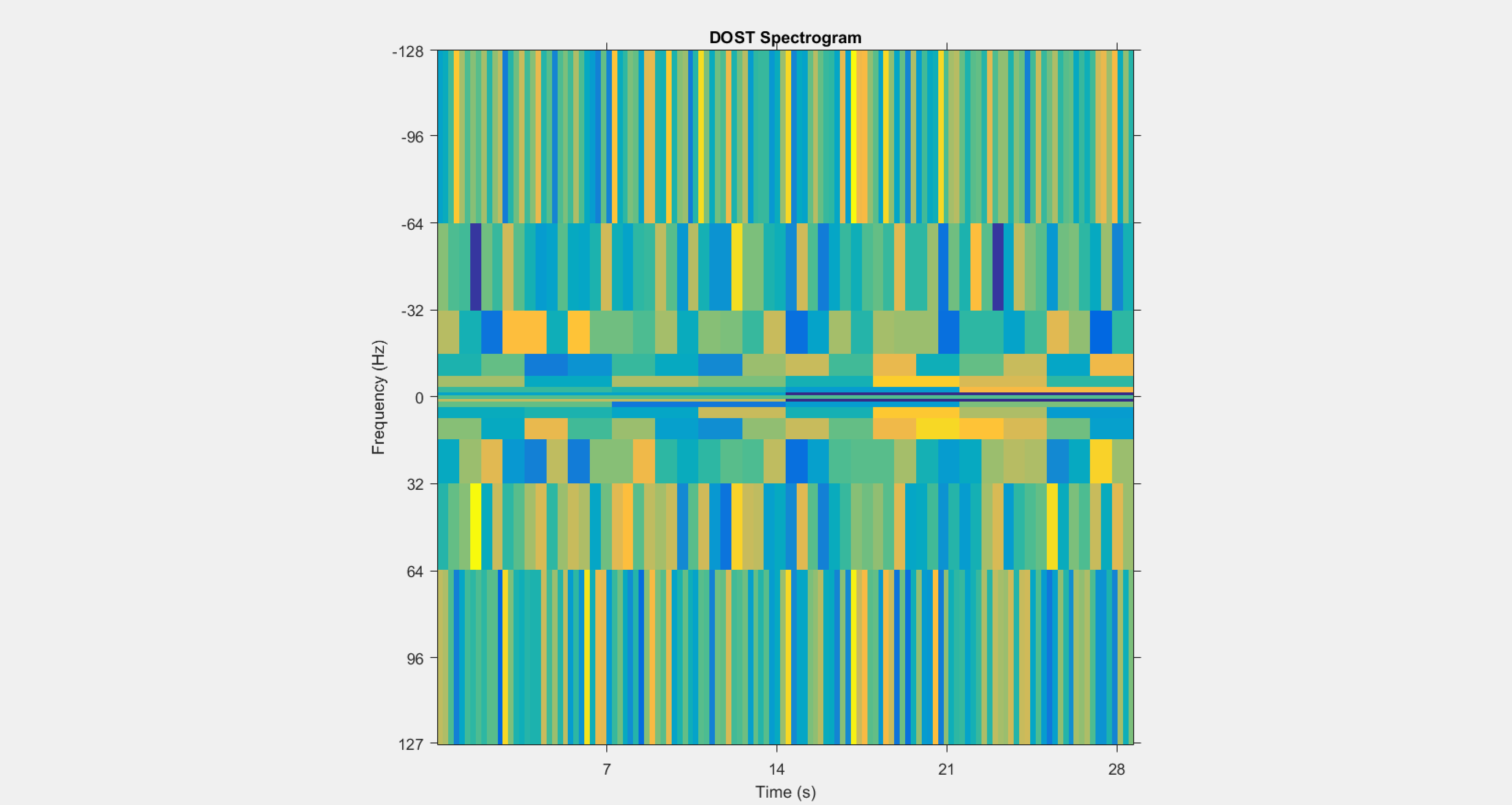
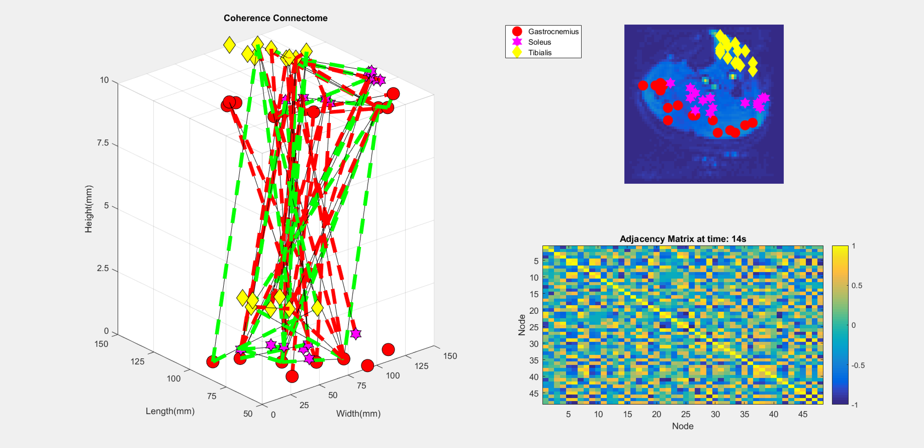
Eight healthy male subjects had their right legs scanned after resting for 30 minutes to normalize the flow of blood in the leg. Acquisition was performed using a 16 channel T/R extremety coil and a General Electric Healthcare MR750 3T MRI. Anatomical reference scans, as seen in Figure 1, were acquired using a fat suppressed PD-weighted scan (voxel size = 0.625x0.625x4mm, 15 slices, 1mm gap, TE/TR = 30ms/3000ms, and flip angle = 111 degrees). Resting state BOLD scans were acquired with the following parameters: voxel size = 2.5x2.5x10mm, 2 slices, no gap, TE/TR = 35ms/109ms, flip angle = 70 degrees, 2434 temporal points. BOLD motion correction was performed using the FMRIB Software Library (FSL). For each scan, binary masks were generated for each of the muscles of interest (Gastrocnemius, Soleus, Tibialis Anterior) using FSL and MATLAB. The graph for each subject was generated with 24 nodes with an equal number of nodes randomly distributed between each muscle. As seen in Figure 2, 256 points of the time series data, from each node, was then used as a basis from which the other dimensions were derived. The graph was then filled along the two dimensions of interest; a coherence and a fractal dimension. The coherence was calculated by performing the Discrete Orthogonal Stockwell Transform (DOST) ^5,6 on the time series data for each node; the output spectrogram showing the change in signal frequency spectra over time is shown in Figure 3. Column-wise correlation of the spectrogram of node A with that of node B results in the coherence as a function of time, and is assigned as the edge weightings in the coherence dimension. This is shown in Figure 4, where the constructed connectome is shown on the left, with coherences being represented as edge diameters. Similarly, the node weightings for the fractal dimensions were calculated by first windowing the time series for each node, then computing the Higuchi Fractal Dimension for each window ⁷. The fractal dimension edge weightings were then recorded as the differences between the nodes over time. The connectome is shown in Figure 5. This investigation looked to compare the functional data extracted by the graphs to the structural physiology the graph is based upon. As the nodes are distributed within three muscles, the edges then fall under two categories of connections. Category A is divided into intermuscular and intramuscular. Edges that connect two nodes within the same muscle are categorized as inter- muscular and those between different muscles as intramuscular. Additionally for category B, the edges can be further subdivided into the specific muscles they connect, resulting in six connection subcategories; G-G, G-S, G-T, S-S, S-T, T-T. Where G, S, and T stand in for Gastrocnemius, Soleus, and Tibialis Anterior respectively. These categories are then used as groupings to assess if any functional distinction between the structural groups can be depicted.

Results and Discussion

The constructed graph is shown in Figures 4 and 5 with only edge values over certain threshold being shown. Edge connections for a dimension at any time point can effectively represent as a skew symmetric adjacency matrix. As the graph is constructed over two dimensions; both can be viewed separately. Due to the information of interest, the edge data, being comprised of paired data; classical analysis of variance (ANOVA) testing is not a valid test as the assumption of independent samples is broken. The data was assessed using a Generalized Linear Mixed-Effects (GLME) Model. The model follows the Wilkinson notation for describing regression and repeated measures models (i.e. Domain -1+CategoryA*CategoryB-Subject) ⁷, where the model fits for the dimensional data while taking into account the combination and individual effects of both the aforementioned edge categories A and B. The model fits the coherence domain significantly with p<0.0013; the fractal domain could not be fit as the non- normal data distribution breaks assumptions of the model. Further development of GSP could prove to open new avenues of processing muscle BOLD data. GSP’s uses extend to multi-modal data; mBOLD and electromyography ⁸ have been used in conjunction and could stand to benefit from GSP. GSP also has multiscale applications; allowing for analysis of localized and distributed clusters of nodes throughout the body within are larger graph.

Acknowledgements

No acknowledgement found.