1125
Deep Learning Based Mask Generation Tools for QSM1Division of Biomedical engineering, Hankuk University of Foreign Studies, Yongin-si, Gyeonggi-do, Korea, Republic of, 2Imaging institute, Cleveland Clinic Foundation, Cleveland, OH, United States, 3AIRS Medical, Seoul, Korea, Republic of
Synopsis
Even subtle differences in masks can generate systematic but avoidable errors in QSM calculations. We believe these errors propagate through the calculation of the background phase. In this work, we assessed the effect of the mask on the QSM, selected optimal mask generation method and Deep Learning-based efficient mask generation method for in-vivo has been presented. This study represents the first step towards a fully-automated and optimal workflow for QSM calculation.
Introduction
Several studies have shown that quantitative susceptibility mapping (QSM) is a candidate biomarker for neurological disorders such as Parkinson’s Disease, Multiple Sclerosis and Alzheimer’s Disease 1-3.QSM is reconstructed from the phase of gradient echo images(GRE). This reconstruction is notoriously ill-posed4. The basic steps in QSM reconstruction are phase unwrapping, background phase removal, and calculation of magnetic susceptibility.
Removal of the background phase is particularly problematic and depends sensitively on separating the background from tissue with a brain tissue mask. However, mask generation methods have not been standardized for QSM. Systematic study of the effects of mask generation methods on QSM reconstruction has not, to our knowledge, been performed.Researchers use various methods for mask generation, such as FSL BET5, STI Suite6 and manual tracing. Because each mask generation method utilizes a different algorithm and inclusion/exclusion criteria, the masks differ. As a result, there is variation in the QSM results that depend solely on the choice of mask. Such variability can interfere with valid interpretation in a clinical setting. Therefore, a method for optimal mask generation method is needed for accurate QSM.
In this work, 1) the effect of mask on the QSM is assessed, 2) based on it, optimal mask generation method is selected and 3) Deep Learning (DL) based efficient mask generation method for in-vivo has been proposed. The QSM with optimized mask reveal substantially improved image quality, demonstrating potential for clinical use.
Methods
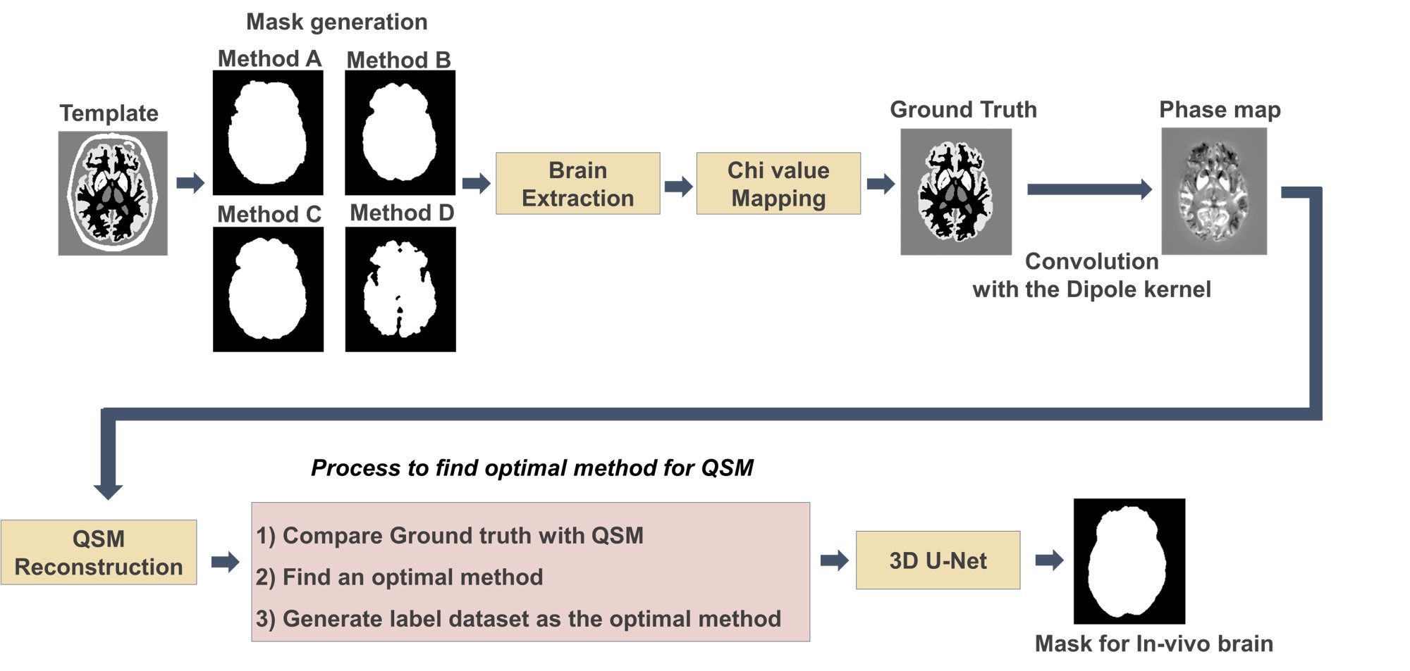
Digital phantomTo investigate the effects of the tissue mask in QSM reconstruction and determine optimal mask generation, we performed digital phantom experiments using the Zubal MRI head phantom7. Magnetic susceptibility values were mapped to the phantom following the values reported by Karsa et al.8. Phase data was generated by convolution with the dipole kernel.
We compared four different mask generation methods: manual tracing, FSL BET, FSL BET with pixel dilation and STI Suite.
Manual tracing masks were defined from 3-dimensional images by two trained raters following guidelines by Tamraz et al.9 and Lim et al.10 . The threshold value of FSL BET was set empirically to the value of 0.5. Pixel dilation was performed by a disk-shaped kernel with a one-voxel radius.
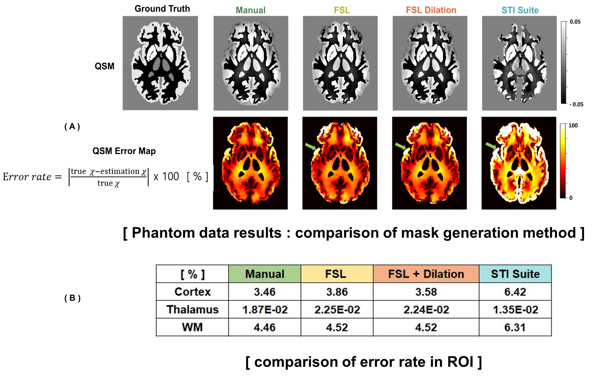
The local field map of phantom data was generated by the V-sharp method11, and QSM is reconstructed by iLSQR12. To find the best mask generation method, error rates between ground truth and recalculated QSM from masks in cortex, white matter, thalamus, and globus pallidus were compared.
Deep Learning
An overview of the deep learning approach is in Figure 1. The OASIS dataset13, consisting of 150 subjects, was used for training data and validation data. Label dataset was generated as the most optimal method investigated in the phantom experiment.
This network was trained with patch-based learning with a patch size of 128x128x64 and 3D U-net architecture. Dice-loss and Adam-w are utilized for updating network parameters. Data augmentation is also applied with Scale Intensity, Random Flip, Randp, Crop, Random Affine transform, Adding Gibbs noise, and Gaussian Smoothing.
The trained network is evaluated with hemorrhagic patient data scanned on 3T (Philips, IRB approved). The patient data were acquired with 0.43x0.43x2mm3 voxels. Images were resampled to the isotropic 1x1x1mm3 voxels by applying crop and padding. For in-vivo, the QSMnet+ 14 was used for QSM map reconstruction.
Results
Phantom studyFigure 2 shows the result from the digital phantom. Figure 2A shows error maps. Error is highest in regions such as the Sylvian fissure (green arrow). The STI Suite mask eroded noticeably more tissue than the other methods, leading to a high error. Figure 2B shows mean errors in each ROI. The manual tracing mask shows the lowest error, overall.
Deep Learning Approach
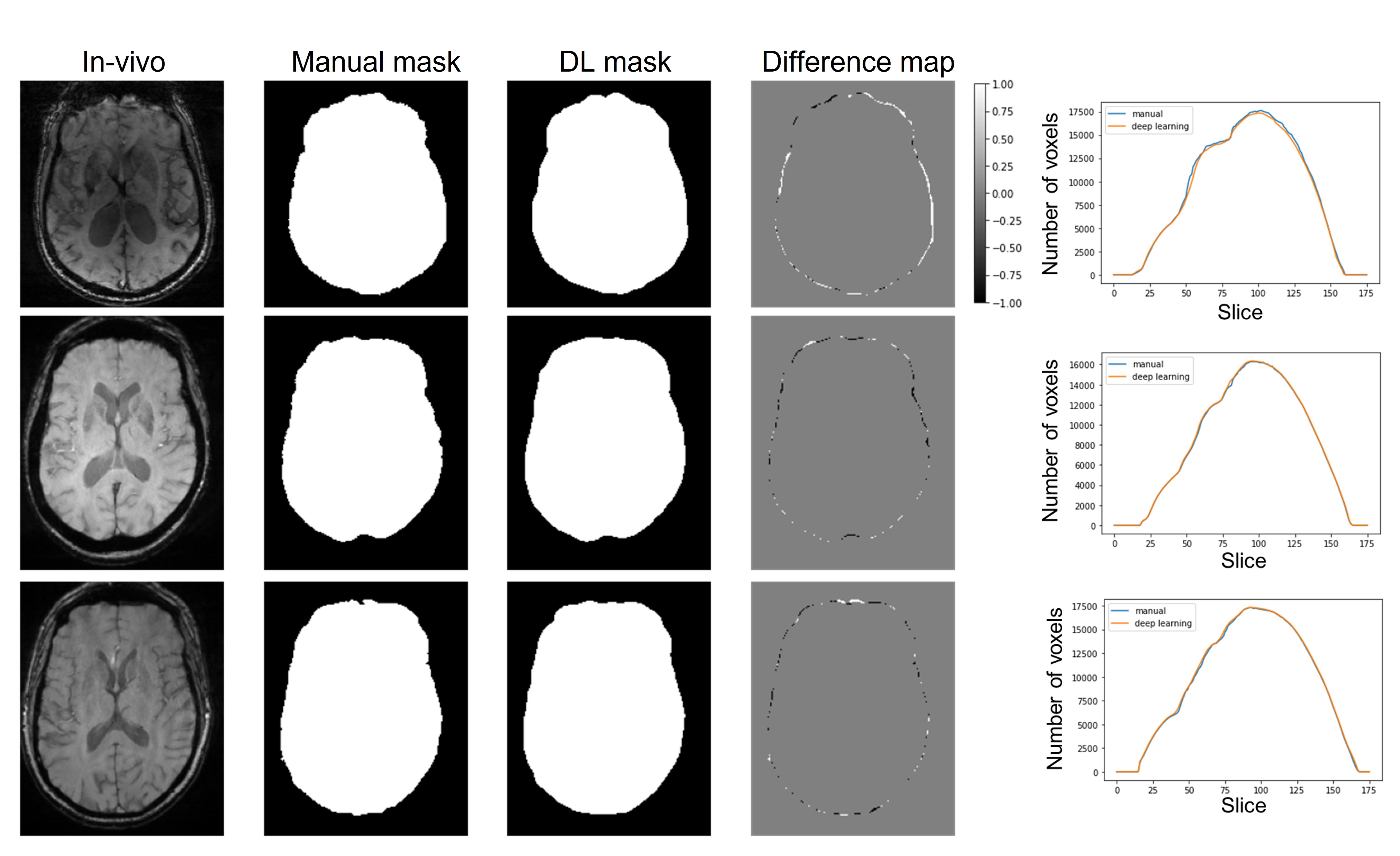
In the phantom experiment, we found that the manual tracing method was optimal. Therefore, we trained the network with a manual segmentation dataset. Figure 3 shows the difference map between validation results of trained network and manual training masks and the comparison graph of number of voxels for each mask. Masks generated by the DL approach match the manually segmented masks closely, albeit with a smoother edge. The number of voxels in each slice is plotted together. It shows DL-based mask has similar to manual tracing results and the differences are negligible
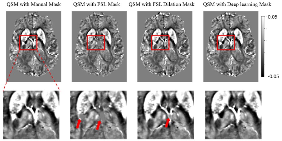
In figure 4 shows results from the OASIS dataset. As compared with results generated with a manually segmented mask, susceptibility values associated with the FSL-generated masks are systematically low in the central vein area (red arrows), while values associated with the deep learning-generated mask match closely.
Patient Data
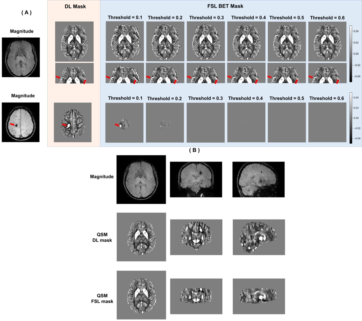
Figure 5 shows QSM maps from a hemorrhagic patient. Results using FSL mask with various thresholds are presented together. Figure 5 shows different QSM maps varying on mask generation methods. Also, Compared to DL-based method, the FSL BET mask shows eroded noticeably in the upper brain area.
Conclusions & Disscusions
This study represents the first step towards a fully-automated and optimal workflow for QSM calculation. Even subtle differences in masks can generate systematic but avoidable errors in susceptibility calculations. We believe these errors propagate through the calculation of the background phase. Future work will entail an end-to-end calculation of QSM images within the deep learning framework.Acknowledgements
This work was supported by the National Research Foundation of Korea (NRF) grant funded by the Korea government (MSIT) (NRF-2020R1A2C4001623)
References
1. Langkammer, C., et al (2016). Quantitative susceptibility mapping in Parkinson’s disease. PLoS One, 11(9), e0162460.
2. Chen, W., et al (2014). Quantitative susceptibility mapping of multiple sclerosis lesions at various ages. Radiology, 271(1), 183-192.
3. Acosta-Cabronero, et al (2013). In vivo quantitative susceptibility mapping (QSM) in Alzheimer’s disease. PloS one, 8(11), e81093.
4. Li, L., & Leigh, J. S. (2004). Quantifying arbitrary magnetic susceptibility distributions with MR. Magnetic Resonance in Medicine: An Official Journal of the International Society for Magnetic Resonance in Medicine, 51(5), 1077-1082.
5. Smith, S. M. (2002). Fast robust automated brain extraction. Human brain mapping, 17(3), 143-155.
6. Li, W., Avram, A. V., Wu, B., Xiao, X., & Liu, C. (2014). Integrated Laplacian‐based phase unwrapping and background phase removal for quantitative susceptibility mapping. NMR in Biomedicine, 27(2), 219-227.
7. Zubal, I. G., Harrell, C. R., Smith, E. O., Rattner, Z., Gindi, G., & Hoffer, P. B. (1994). Computerized three‐dimensional segmented human anatomy. Medical physics, 21(2), 299-302.
8. Karsa, A., Punwani, S., & Shmueli, K. (2019). The effect of low resolution and coverage on the accuracy of susceptibility mapping. Magnetic resonance in medicine, 81(3), 1833-1848.
9. Tamraz, J. C., Comair, Y. G., & Tamraz, J. C. (2004). Atlas of regional anatomy of the brain using MRI. Springer-Verlag.
10. Lim, I. A. L., Faria, A. V., Li, X., Hsu, J. T., Airan, R. D., Mori, S., & van Zijl, P. C. (2013). Human brain atlas for automated region of interest selection in quantitative susceptibility mapping: application to determine iron content in deep gray matter structures. Neuroimage, 82, 449-469.
11. Li, W., Wu, B., & Liu, C. (2011). Quantitative susceptibility mapping of human brain reflects spatial variation in tissue composition. Neuroimage, 55(4), 1645-1656.
12. Li, W., Wang, N., Yu, F., Han, H., Cao, W., Romero, R., ... & Liu, C. (2015). A method for estimating and removing streaking artifacts in quantitative susceptibility mapping. Neuroimage, 108, 111-122.
13. LaMontagne, P. J., Benzinger, T. L., Morris, J. C., Keefe, S., Hornbeck, R., Xiong, C., ... & Marcus, D. (2019). OASIS-3: longitudinal neuroimaging, clinical, and cognitive dataset for normal aging and Alzheimer disease. MedRxiv.
14. Jung, W., Yoon, J., Ji, S., Choi, J. Y., Kim, J. M., Nam, Y., ... & Lee, J. (2020). Exploring linearity of deep neural network trained QSM: QSMnet+. Neuroimage, 211, 116619.Figures