Introduction

Magnetic Resonance Spectroscopic Imaging (MRSI) is an emerging medical imaging modality, which is steadily gaining popularity. It allows the acquisition of spectra, which encode the biochemical substances, for each voxel. Compared to other imaging techniques such as Magnetic Resonance Imaging (MRI) its acquisition time is relatively long. This makes its clinical application challenging. The typical approach to decrease the acquisition time is to omit k-space sampling points or trajectories. These are then later computationally reconstructed. In this paper a graph neural network is proposed for the reconstruction of undersampled concentric ring k-space data.

Methods

Non-water suppressed whole-brain MRSI data were collected from seven volunteers in ten random head positions. The data of the first six volunteers were used for training and the data of the last volunteer for validation. Water-suppressed, long-TR FID-MRSI data were measured from all volunteers in the tenth position, and was used to evaluate the network. In each scan concentric ring trajectories were used, in total 16 rings with 388 points per ring each are acquired. Graphs are defined by connecting point pairs with a distance less than 1.5 times the Nyqusit criterion. These rings are undersampled, by fully sampling the inner 6 and then skipping every second of the outer rings.The proposed complex Graph Neural Network (GNN) consists of two graph convolutional layers with a tanh activation function in between. A novel graph convolutional layer is introduced. For this purpose indicator functions are applied
$$
\begin{aligned}
&\chi_\epsilon: \mathbb{R} \rightarrow \mathbb{R} \\
&x \mapsto
\begin{cases}
1 & \text{if} ~|x| < \epsilon \\
0 & \text{else}
\end{cases}
\end{aligned}
$$
The resulting weighting function $$$\omega:\mathbb{R}^n \rightarrow \mathbb{R}$$$is then defined as

$$
\omega(u(v,w)) = \chi_\epsilon(u(v,w) - \mu),
$$
where $$$\epsilon$$$ and $$$\mu$$$ are learnable parameters. Following the framework by Monti etal⁴ the patch operator is defined as
$$
\begin{equation}
D_j(v)f = \frac{1}{C_{v,j}} \sum_{w \in N(v)} \omega_j(u(v,w))f(w), ~ j = 1,...,J,
\end{equation}
$$
where
$$
\begin{equation}
C_{v,j} = \sum_{w \in N(v)} \omega_j(u(v,w))
\end{equation}
$$
In general, the patch operator can be interpreted as taking the mean of all feature vectors close to a certain location. $$$J$$$ represents the number of patches that are extracted.

Due to the complicated structure of the graph it cannot be guaranteed that for every patch operator there is a feature vector located at a favorable position, i.e. $$$C_{v,j} = 0$$$. Therefore, it is necessary to know if a patch has been activated ($$$C_{v,j} > 0$$$). This is done using another indicator function
$$
\begin{equation}
\begin{aligned}
&\chi_{\mathbb{R}>\alpha}: \mathbb{R} \rightarrow \mathbb{R} \\
&x \mapsto
\begin{cases}
1 & \text{if} ~x < \alpha \\
0 & \text{else}
\end{cases}
\end{aligned}
\end{equation}
$$
The activity of a patch at a certain vertex is then given by
$$
\begin{equation}
\text{act}_{v,j} = \chi_{\mathbb{R}>\alpha}(C_{v,j}),
\end{equation}
$$
where $$$\alpha$$$ is a learnable parameter. In the GRAPPA algorithm, the feature vectors are merged with a complex fully-connected layer $$$L_\mathbb{C}: \mathbb{C}^{(J \times m)} \rightarrow \mathbb{C}^m$$$. Here it must be considered that the number of activated patches may vary. Hence, multiple points mapped to the same position can simply be averaged³. The patch vectors are then merged as follows
$$
\begin{equation}
f'(v) = A_v L_\mathbb{C}(\text{act}_{v,1}D_1(v)f, ...,\text{act}_{v,J}D_J(v)f)
\end{equation}
$$
where
$$
\begin{equation}
A_v = \text{max}(\frac{1}{\sum_{j=1}^J \text{act}_{v,j}}, 1)
\end{equation}
$$
and $$$f':V\rightarrow\mathbb{C}^m$$$ is the output of the convolutional layer.

The reconstruction of the presented model is compared against the ground truth (i.e., no undersampling) and a more established reconstruction method. A GRAPPA algorithm, which was specifically developed for concentric rings by Moser et al¹, was implemented.
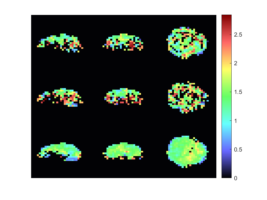
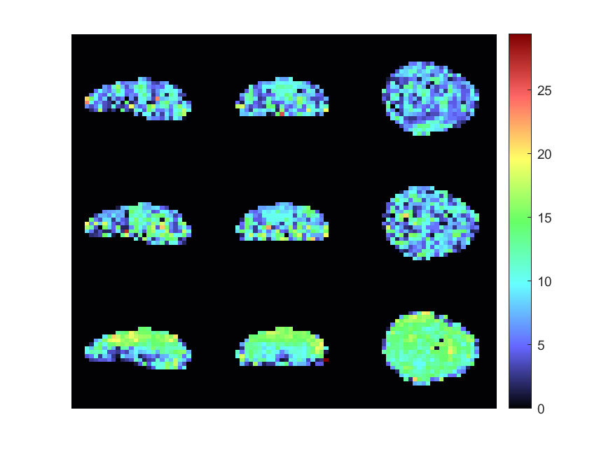
The considered metabolite groups are (tCr [total creatine], tNAA [N- acetylaspartate + N- acetylaspartyl glutamate], and tCho [total choline]). The ratio maps of tNAA to tCho and tCr to tCho are computed and plotted. The Signal-Noise-Ratio (SNR) is given by the LCModel² output.

Results

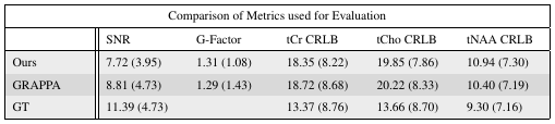
The metabolic maps of tCho to tCr and tNAA to tCr are shown in figures 1 and 2. Here the estimated relative amplitude of each voxel is shown, if its CRLB is lower than 40\%. Althought the average CRLBs of our method and GRAPPA (Figure 4) do not differ dramatically, it can be seen that a our methods leads to a more stable reconstruction of these metabolite maps. The reconstruction of our method still leads to ring-like artifacts in the relative amplitude maps, but compared to GRAPPA, is less noisy.Our method leads to a slight decrease in SNR, compared to GRAPPA. The average SNR of the volume is 7.72 and 8.81 (Figure 4) for our method and GRAPPA. As before, the same ring-like artifact can be observed. The SNR decreases along the edges of the ring.

Discussion and Conclusion

A novel deep learning based method for the reconstructon of undersampled non-Cartesian MRSI data is presented. The introduced model is compared against a state-of-the-art GRAPPA reconstruction algorithm and results in similar reconstructions. Overall, the results suggest that a deep learning based reconstruction is promising, but further research should be done.

Acknowledgements

Austrian Science Fund (FWF): P 35189 \& P 34198-N, Vienna Science and Technology Fund (WWTF): LS20-065