1048
Evaluating Within-Subject Test-Retest Replicability of Free-Water Corrected and Uncorrected Multi-Shell Diffusion MRI Measures.1Imaging, Cleveland Clinic Lou Ruvo Center for Brain Health, Las Vegas, NV, United States, 2Harvard Medical School, Boston, MA, United States
Synopsis
Free-water (FW) estimation could be improved with higher spatial resolution diffusion MRI (dMRI) data acquired at multiple shells. However, the effect of multi-shell protocol features on the accuracy of estimating FW and FW-corrected fractional anisotropy (FA) across the brain structures is currently unknown. We evaluated test-retest reproducibility of FW and FW-corrected FA across 20 major white-matter tracts across four dMRI protocols, two protocols with ADNI-3 and two protocols with HCP sequences. Our analysis suggests higher spatial resolution HCP-style dMRI data acquisition with correction of FW-estimation could be reliably performed in routine clinical investigations.
Introduction
Single-tensor (ST)-derived fractional anisotropy (FA) measures that are estimated in routine clinical investigations are biased not only due to the presence of crossing-fibers1 but also due to the contamination from cerebrospinal fluid (CSF)2. Such CSF-contamination can be corrected by fitting a bi-tensor model3 to account for free water (FW) contamination. FW imaging is widely used currently and has improved our understanding of various neurodegenerative4 and neuropsychiatric disorders5. With the widespread usage of multiband diffusion MRI (dMRI) data acquisition6, it is now possible to acquire higher spatial resolution dMRI data across multiple shells within a reasonable scan time that could improve the estimation of FW in the brain voxel7,8. However, the effect of multi-shell protocol features on the accuracy of estimating FW and FW-corrected FA across the brain structures is currently unknown. Hence, in this study, we collected dMRI data across 4 protocols: the (1) advanced and (2) basic ADNI-3 protocols9, and an HCP dMRI protocol10 with custom diffusion encoding directions (DEC) collected at (3) high (1.5mm3) and (4) a conventional (2mm3) spatial resolution. We evaluated test-retest reproducibility of FW and FW-corrected FA across 20 major WM tracts11 across the four dMRI protocols.Methods
A 32-year-old healthy male participant was scanned over five weeks with the following dMRI protocols on a 3T Siemens Skyra scanner in the same session. Protocol 1 (Advanced ADNI-3): 114 DEC and 13 non-diffusion weighted (b0) images interspersed between the DEC, Multiband factor=3, GRAPPA=2, TR=5000ms, TE=98ms, resolution=2mm3, 3 b-values: 500s/mm2, 1000s/mm2, and 2000s/mm2, and phase-encoding directions of P>>A; opposite phase-encoding (A>>P) b0 image. Acquisition time: 11:37 minutes. Protocol 2 (Basic ADNI-3): 48 DEC and 7 non-diffusion weighted (b0) images interspersed between the DEC, b-value= 1000s/mm2, GRAPPA=2, TR=10700ms, TE=80ms, resolution=2mm3, and phase-encoding directions of P>>A; opposite phase-encoding (A>>P) b0 image. Acquisition time: 11:04 minutes. Protocol 3 (Custom multi-shell): 213 DEC and 25 non-diffusion weighted (b0) images interspersed between the DEC, Multiband factor=3, GRAPPA=2, TR=5218ms, TE=100ms, resolution=1.5mm3, 3 b-values: 500s/mm2, 1000s/mm2, and 2500s/mm2, and phase-encoding directions of P>>A; opposite phase-encoding (A>>P) b0 image. Acquisition time: 23:13 minutes. Protocol 4 (Custom multi-shell): 213 DEC and 25 non-diffusion weighted (b0) images interspersed between the DEC, Multiband factor=3, GRAPPA=2, TR=4200ms, TE=96ms, resolution=2mm3, 3 b-values: 500s/mm2, 1000s/mm2, and 2500s/mm2, and phase-encoding directions of P>>A; opposite phase-encoding (A>>P) b0 image. Acquisition time: 18:41 minutes. A total of four dMRI scans were acquired each week with each protocol, and the process was repeated for five weeks (total: 5x4=20 scans) to evaluate the test-retest reproducibility. Single shell basic ADNI-3 sequence was only acquired to see the effect of FW estimation across single and multi-shell dMRI data. Processing: Every dataset was corrected for EPI distortion and a measure of head motion was computed using eddy12 tool in FSL. The average head motion for all runs was less than the respective protocol’s slice thickness. ST dMRI-derived measures were estimated using dtifit tool of FSL, and (ii) FW and FW-corrected ST dMRI measures were obtained using the original Matlab implementation3 (Matlab) and DiPY implementation of multi-shell dMRI acquisition13 (DiPY). Of note, since FA and its derivatives are only reliable at b<=1000s/mm2, estimation of ST FA and FW-corrected FA was only done using b-values<=1000s/mm2 for protocols 1, 3, and 4. TBSS14 protocol was used to register ST FA maps, FW maps, and FW-corrected FA maps obtained across the five runs for each protocol independently to MNI152 and upsampled to 1mm3. JHU WM atlas of 20 major WM tracts pre-registered to MNI152 was then used as a mask to obtain ST FA, FW, and FW-corrected FA at each WM tract, and the coefficient of variance (CoV) was computed across each protocol.Results
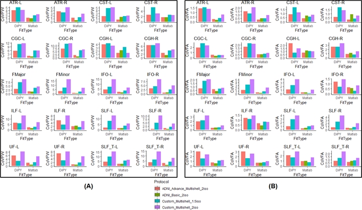
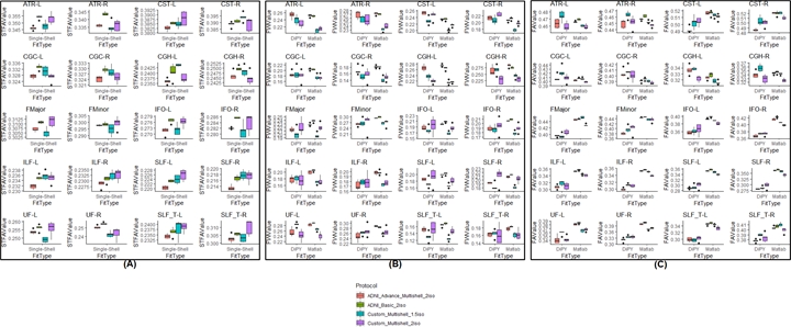
FW estimated using Matlab had a mean CoV=2.78±1.09 across all the protocols with the least CoV for Protocol-2 (CoV=1.31±0.54) and the maximum CoV for Protocol-4 (CoV=4.98±1.83) (Fig.1A) while FW estimated using DiPY had a mean CoV=6.71±2.86 across all the protocols with the least CoV for Protocol-1 (CoV=4.31±1.85) and the maximum CoV for Protocol-4 (CoV=9.66±4.15) (Fig.1A). FW-corrected FA estimated using Matlab had a mean CoV=0.75±0.29 across all the protocols with the least CoV for Protocol-1 (CoV=0.57±0.2) and the maximum CoV for Protocol-4 (CoV=1.12±0.44) while FW-corrected FA estimated using DiPY had a mean CoV=2±0.86 across all the protocols with the least CoV for Protocol-1 (CoV=1.57±0.74) and the maximum CoV for Protocol-4 (CoV=2.57±1.14) (Fig.1B). Despite similar FW estimated for almost all major WM tracts for both Matlab and DiPY (Fig.2B), DiPY estimation consistently provided lower FW-corrected FA (Fig.2C).Discussion and Conclusion
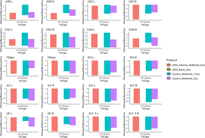
Our analysis suggests higher spatial resolution HCP-style dMRI data acquisition with correction of FW-estimation could be reliably performed in routine clinical investigations and either Matlab or DiPY could be used to estimate FW and FW-corrected dMRI measures. However, since Matlab and DiPY yield approximately 20% difference in the estimated FW-corrected FA value (Fig.3), the analytic techniques should not be combined.Acknowledgements
This study is supported by the National Institutes of Health (grant R01NS117547, P20GM109025, R01NS118760, and R01NS118760-S1) and the Keep Memory Alive-Young Investigator Award (Keep Memory Alive Foundation).References
1. Jeurissen B, Leemans A, Tournier J-D, Jones DK, Sijbers J. Investigating the prevalence of complex fiber configurations in white matter tissue with diffusion magnetic resonance imaging. Hum Brain Mapp. United States; 2013;34:2747–2766.
2. Papadakis NG, Martin KM, Mustafa MH, et al. Study of the effect of CSF suppression on white matter diffusion anisotropy mapping of healthy human brain. Magn Reson Med. United States; 2002;48:394–398.
3. Pasternak O, Sochen N, Gur Y, Intrator N, Assaf Y. Free water elimination and mapping from diffusion MRI. Magn Reson Med. United States; 2009;62:717–730.
4. Bergamino M, Walsh RR, Stokes AM. Free-water diffusion tensor imaging improves the accuracy and sensitivity of white matter analysis in Alzheimer’s disease. Sci Rep. 2021;11:6990.
5. Chang X, Mandl RCW, Pasternak O, Brouwer RM, Cahn W, Collin G. Diffusion MRI derived free-water imaging measures in patients with schizophrenia and their non-psychotic siblings. Prog Neuro-Psychopharmacology Biol Psychiatry. 2021;109:110238.
6. Sotiropoulos SN, Jbabdi S, Xu J, et al. Advances in diffusion MRI acquisition and processing in the Human Connectome Project. Neuroimage. 2013/05/20. 2013;80:125–143.
7. Mishra V, Guo X, Delgado MR, Huang H. Towards tract-specific fractional anisotropy (TSFA) at crossing-fiber regions with clinical diffusion MRI. Magn Reson Med. 2015;74:1768–1779.
8. Bergmann Ø, Henriques R, Westin C-F, Pasternak O. Fast and accurate initialization of the free-water imaging model parameters from multi-shell diffusion MRI. NMR Biomed. 2020;33:e4219.
9. https://adni.loni.usc.edu/wp-content/uploads/2017/07/ADNI3-MRI-protocols.pdf.
10. https://www.humanconnectome.org/hcp-protocols-ya-3t-imaging.
11. Wakana S, Caprihan A, Panzenboeck MM, et al. Reproducibility of Quantitative Tractography Methods Applied to Cerebral White Matter. Neuroimage. 2007;36:630–644.
12. Andersson JLR, Sotiropoulos SN. An integrated approach to correction for off-resonance effects and subject movement in diffusion MR imaging. Neuroimage. United States; 2016;125:1063–1078.
13. Hoy AR, Ly M, Carlsson CM, et al. Microstructural white matter alterations in preclinical Alzheimer’s disease detected using free water elimination diffusion tensor imaging. PLoS One. United States; 2017;12:e0173982.
14. Smith SM, Jenkinson M, Johansen-Berg H, et al. Tract-based spatial statistics: Voxelwise analysis of multi-subject diffusion data. Neuroimage. 2006;31:1487–1505.
Figures