0960
Inline artifact identification using segmented acquisitions and deep learning
Keerthi Sravan Ravi1,2, Marina Manso Jimeno1,2, John Thomas Vaughan Jr.2, and Sairam Geethanath2
1Department of Biomedical Engineering, Columbia University, New York, NY, United States, 2Columbia Magnetic Resonance Research Center, New York, NY, United States
1Department of Biomedical Engineering, Columbia University, New York, NY, United States, 2Columbia Magnetic Resonance Research Center, New York, NY, United States
Synopsis
MR artifacts degrade image quality and affect diagnosis, requiring thorough examination by the MR technician, and reacquisition in some cases. We employ a combination of segmented acquisitions and a deep learning tool (ArtifactID) to perform more frequent updates to image quality during acquisition. ArtifactID identified wrap-around, Gibbs ringing and motion artifacts, with a mean accuracy of 99.43%. The segmented acquisitions for rescans resulted in a 12.98% time gain over the full-FOV sequence. In addition, ArtifactID alleviates burden on the MR technician via automatic artifact identification, saving image quality evaluation time and augmenting expertise.
Introduction
MR artifacts such as wrap-around, Gibbs ringing, and motion pose challenges to image quality1,2. They may obscure pathology and can interfere in diagnosis1. Conventionally, the MR technician examines the acquired data to identify any artifacts after each sequence acquisition. This is a time-consuming and skill-demanding task3. If the data is severely artifact-corrupted, the technician re-acquires the entire sequence. This not only results in added acquisition time but also burdens the MR technician to re-analyze images. Therefore, in this work, we propose to partition a sequence into segments and leverage “ArtifactID” to automate inline artifact identification4. The segmented sequences cover adjacent sections of the full field-of-view (FOV), such that the full volume can be obtained by concatenating the segmented data. After the first segment, ArtifactID notifies the technician about the presence of artifacts, allowing the acquisition parameters to be adjusted for the following segments, saving time and reducing data loss (Figure 1). The goal of this work is to employ segmented acquisitions and deep learning based automatic artifact identification to minimize re-acquisition events and reduce rescan time.Methods
We leveraged vendor-supplied sequences for the full-FOV and segmented acquisitions on GE 3.0T Signa Premier and Siemens 3.0T Prisma Fit scanners. The full-FOV acquisition was a 3D T1-weighted sequence with FOV=256x256 mm2, N=256x256 and 172 slices, duration=5:12 (minutes:seconds). The slice offsets of the segmented acquisitions were hard-coded to cover a specific section of the entire FOV. Each segment acquired 96 slices, with the same FOV and matrix size, duration=3:01. We acquired wrap-around corrupted data by setting a smaller FOV. Gibbs ringing and motion artifacts were induced via subject motion. To train the artifact identification models, we simulated wrap-around and Gibbs ringing utilizing the publicly available IXI dataset5 (T1 contrast only). Figures 2 (a, b) show representative slices of these simulated artifacts. We changed the data-split and model architecture for Gibbs ringing in comparison to previous work4. We trained a binary classification model based on the ResNet-architecture6. The input was 64x64 randomly cropped standardized ($$$ \mu=0, \sigma^2=1 $$$) total-variation images. The data split was 85-10-5% for training, validation and test sets. We combined data simulated on two motion-free datasets with one motion-corrupted dataset (all T1w prospectively acquired). The data split was the same as Gibbs ringing. The simulation process followed ref. 7 and we utilized the wrap-around model’s architecture4. Figure 2c shows representative slices of the simulated motion artifact. We evaluated the trained models on prospectively acquired T1w segments and obtained Grad-CAM8 heatmaps for true-positive (TP), false-positive (FP), true-negative (TN) and false-negative (FN) inputs. We acquired full-FOV, segment 1, segment 2, segment 1 with wrap-around, and segment 1 with Gibbs and motion artifacts from two healthy volunteers on each scanner. The code is open-source and available on Github9.Results
Training both in-plane and through-plane wrap-around models required 9:00 for 5 epochs for 15,811 and 14,967 slices, respectively. The in-plane model achieved 100% training accuracy and 100% precision/recall. The through-plane model reached 99% training accuracy and 98.8/93.7% precision/recall on the test set. Training the Gibbs ringing model on 10,000 image pairs for 25 epochs required approximately 18:14. The model achieved training/validation accuracies of 98.71%/98.92%. Precision and recall metrics evaluated on test sets was 77.39%/100%. Training the motion model on 152/336 images (no-artifact/motion) for 25 epochs required approximately 56 seconds. The model achieved 100% training and validation accuracies, and 100%/100% precision/recall on the test set. Figures 3-5 show Grad-CAM visualization of TP, TN, FP and FN across both subjects for all three artifacts. For wrap-around, the heatmaps highlight the superposition of anatomies. However, background noise or low intensity wraps leads to misclassifications. For Gibbs ringing, the heatmaps indicate the model’s ability to localize the occurrences. For motion, the model relies on disturbances in the background to identify the artifact. The time saved by employing segmented acquisitions for rescans was 1:21.Discussion and conclusion
The acquisition times for the full-FOV and segmented acquisitions were 5:12 and 6:02, respectively. However, in the case of artifact corruption, the total acquisition time for the full-FOV sequence will be 10:24, versus 9:03 for the segmented acquisitions. The reported time gain does not include the time spent manually examining the images. In this way, ArtifactID alleviates the burden imposed on the MR technician by automating the artifact identification process, saving additional time and augmenting expertise. Therefore, we extended the work in ref. 4 by including motion artifacts and integrating with acquisition. For model explainability purposes, we visualized GradCAM heatmaps. Although the in-plane model’s accuracy indicates overfitting, the TP examples suggest its ability to localize the characteristic superposition of anatomies. This is also true for the through-plane model. The motion artifact simulation on the IXI dataset did not reflect the real-world occurrence, leading to overfitting on the prospective dataset. Future work includes improving the artifact simulation. In conclusion, employing segmented acquisitions and leveraging ArtifactID will allow frequent updates on image quality and artifact presence inline at the scan time.Acknowledgements
This study was funded [in part] by the Seed Grant Program for MR Studies and the Technical Development Grant Program for MR Studies of the Zuckerman Mind Brain Behavior Institute at Columbia University and Columbia MR Research Center site.References
1. Krupa K, Bekiesińska-Figatowska M. Artifacts in magnetic resonance imaging. Polish J Radiol 2015;80:93–106. https://doi.org/10.12659/PJR.892628.2. Smith TB, Nayak KS. MRI artifacts and correction strategies. Imaging Med 2010;2:445–7. https://doi.org/10.2217/iim.10.33.
3. Andre JB, Bresnahan BW, Mossa-Basha M, Hoff MN, Patrick Smith C, Anzai Y, et al. Toward quantifying the prevalence, severity, and cost associated with patient motion during clinical MR examinations. J Am Coll Radiol 2015;12:689–95. https://doi.org/10.1016/j.jacr.2015.03.007.
4. Manso Jimeno M, Ravi KS, Thomas Vaughan Jr. J, Oyekunle D, Ogbole G, Geethanath S. ArtifactID: identifying artifacts in low field MRI using deep learning. Proc. 2021 ISMRM SMRT Virtual Conf. Exhib., 2021.
5. https://brain-development.org/ixidataset/
6. He K, Zhang X, Ren S, Sun J. Deep residual learning for image recognition. Proc. IEEE Comput. Soc. Conf. Comput. Vis. Pattern Recognit., 2016. https://doi.org/10.1109/CVPR.2016.90.
7. Mohebbian M, Walia E, Habibullah M, Stapleton S, Wahid KA. Classifying MRI motion severity using a stacked ensemble approach. Magn Reson Imaging 2021;75:107–15.
8. Selvaraju RR, Cogswell M, Das A, Vedantam R, Parikh D, Batra D. Grad-CAM: Visual Explanations from Deep Networks via Gradient-Based Localization. Proc. IEEE Int. Conf. Comput. Vis., vol. 2017- Octob, 2017, p. 618–26. https://doi.org/10.1109/ICCV.2017.74.
9. https://github.com/imr-framework/artifactID
Figures
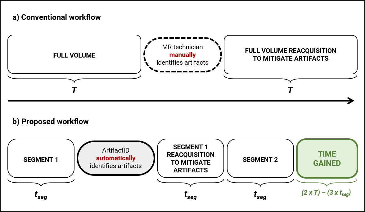
Comparison of conventional and proposed workflows. (a) Conventionally, if severe artifacts are identified, the full-FOV sequence (duration T) has to be repeated. This results in twice the acquisition time (2T). (b) Proposed workflow - a full-FOV sequence is partitioned into two segments (duration tseg). If artifacts are identified, only the corresponding segment has to be repeated (3tseg in total). Therefore, time lost is only the duration of the affected segment.
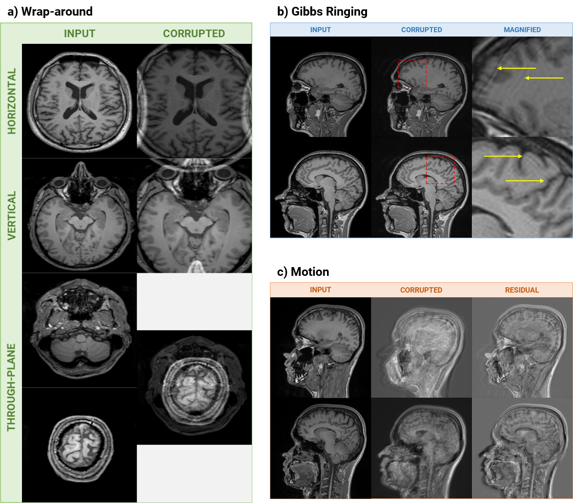
Example outputs of the artifact simulation process. (a) In-plane and through-plane wrap-around artifact axially simulated on the IXI dataset. (b) Gibbs ringing artifact sagittally simulated on the IXI dataset. (c) Motion artifact simulated on prospectively acquired T1-weighted sagittal data.
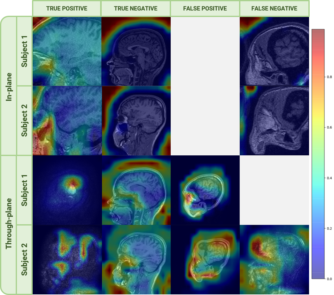
Representative GradCAM heatmaps from a T1-weighted sagittal sequence localizing the occurrences of in-plane and through-plane wrap-around artifacts across both subjects. The wrap-around models were trained on axially oriented T1-weighted images but demonstrated the ability to generalize to other orientations
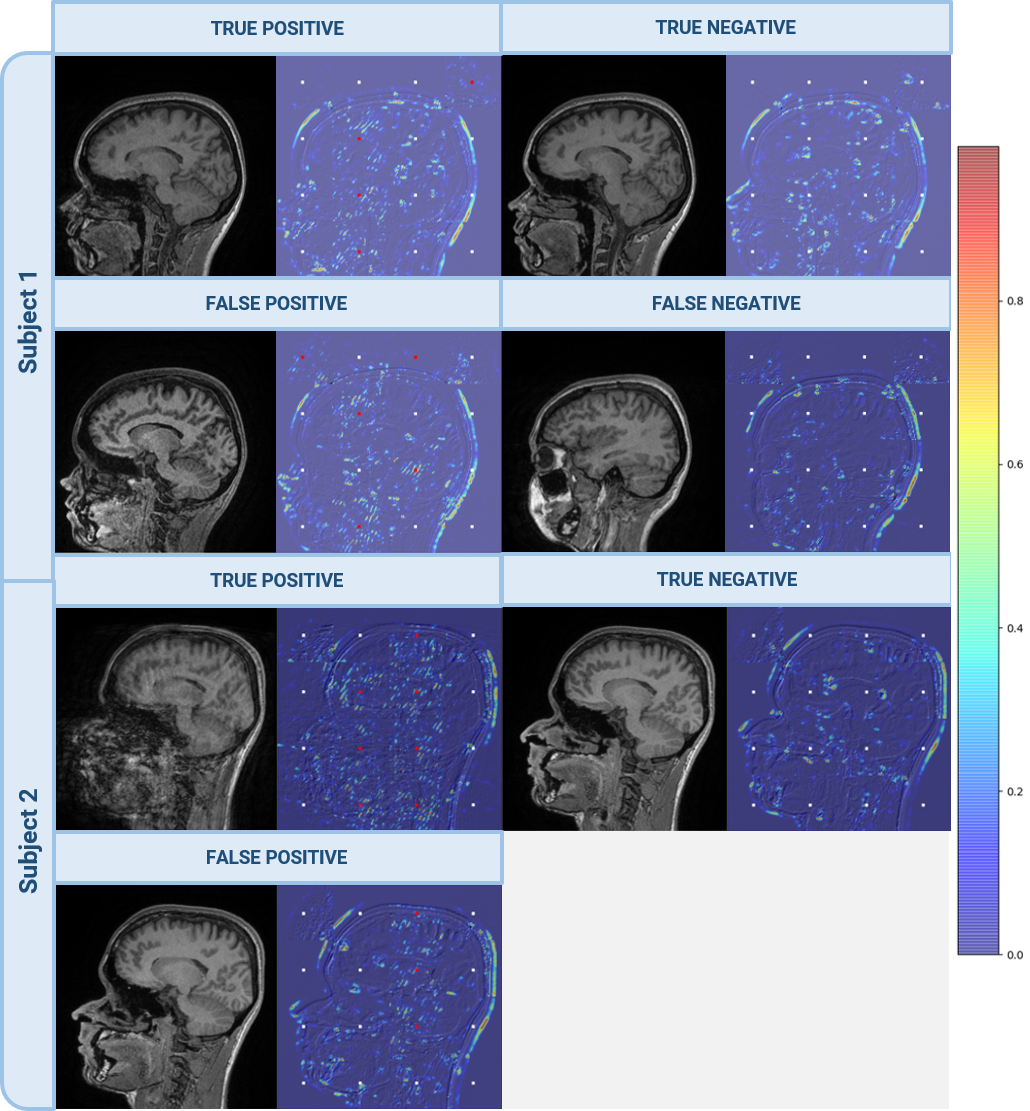
Representative Grad-CAM heatmaps from a T1-weighted sagittal sequence localizing the occurrences of the Gibbs ringing artifact across both subjects. The Gibbs ringing artifact identification model operated on 64x64 patches. Therefore, white and red boxes are overlaid on 64x64 patches of each input slice indicating the absence or presence of the Gibbs ringing artifact.

Representative Grad-CAM heatmaps from a T1-weighted sagittal sequence localizing the occurrences of the motion artifact across both subjects.
DOI: https://doi.org/10.58530/2022/0960