INTRODUCTION

Time-resolved 3D phase-contrast (PC) MRI, also called 4D flow MRI, is a promising technique to retrospectively evaluate flows inside a 3D volume. Thereby hemodynamic parameters such as peak velocity and flow rates, along with derived biomarkers, e.g., wall shear stress, turbulent kinetic energy, become accessible in a non-invasive way¹. However, its development in clinical routine remains limited by the long scan times. To decrease the scan duration, techniques like parallel imaging have been developed.
In this study, two acceleration methods, GRAPPA (R=3) and compressed sensing (R=7.6), were investigated together with a fully-sampled k-space 4D flow acquisition. The experiment was conducted in a well-controlled setup under pulsatile inflow regime presenting complex flow features characteristic of the cardiovascular system. A Computational Fluid Dynamics (CFD) simulation was also performed under the same conditions and used as a third-party reference to characterize the differences.

METHODS

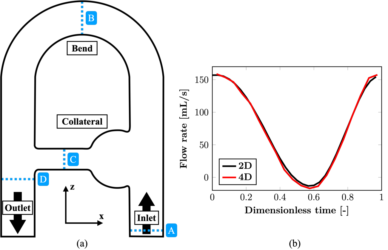
The rigid phantom setup used to acquire the 4D flow MRI data is presented in the coronal (xz-)plane in Figure 1. The circuit was supplied with a Newtonian blood-mimicking fluid following a sinusoidal pulsatile flow rate imposed at the phantom inlet. The investigated acquisition methods were a complete k-space sampling (fully-sampled, FS), GRAPPA R=3 (G3) and compressed sensing (CS, prototypal sequence) R=7.6 at 1.5 T (MAGNETOM Sola, Siemens Healthcare, Erlangen, Germany). Isotropic 2mm³ voxels were set with TE=3.70-4.15 ms, temporal resolution =48.3-51.8 ms, simulated cardiac R-R interval =1 s, 20 (FS, G3) or 25 (CS) reconstructed cardiac phases and encoding velocities (VENC) =0.7 m/s in-plane and 0.2 m/s through-plane. All MR images went through an in-house post-processing procedure to correct for through-plane geometric distortion, noise masking and phase unwrapping.
CFD simulation was conducted using the YALES2BIO solver (https://imag.umontpellier.fr/~yales2bio/) on the same computer-aided design (CAD) geometry². The velocity at the inlet boundary was prescribed from 2D cine PC-MRI measurements. In order to compare both techniques, the CFD velocity fields were phase-averaged and downsampled to the MRI spatial resolution³. These low-resolution fields are referred to as CFD,LR. Finally, MRI volumes were registered onto the computational model.

RESULTS

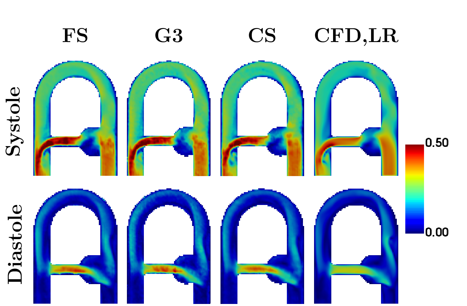
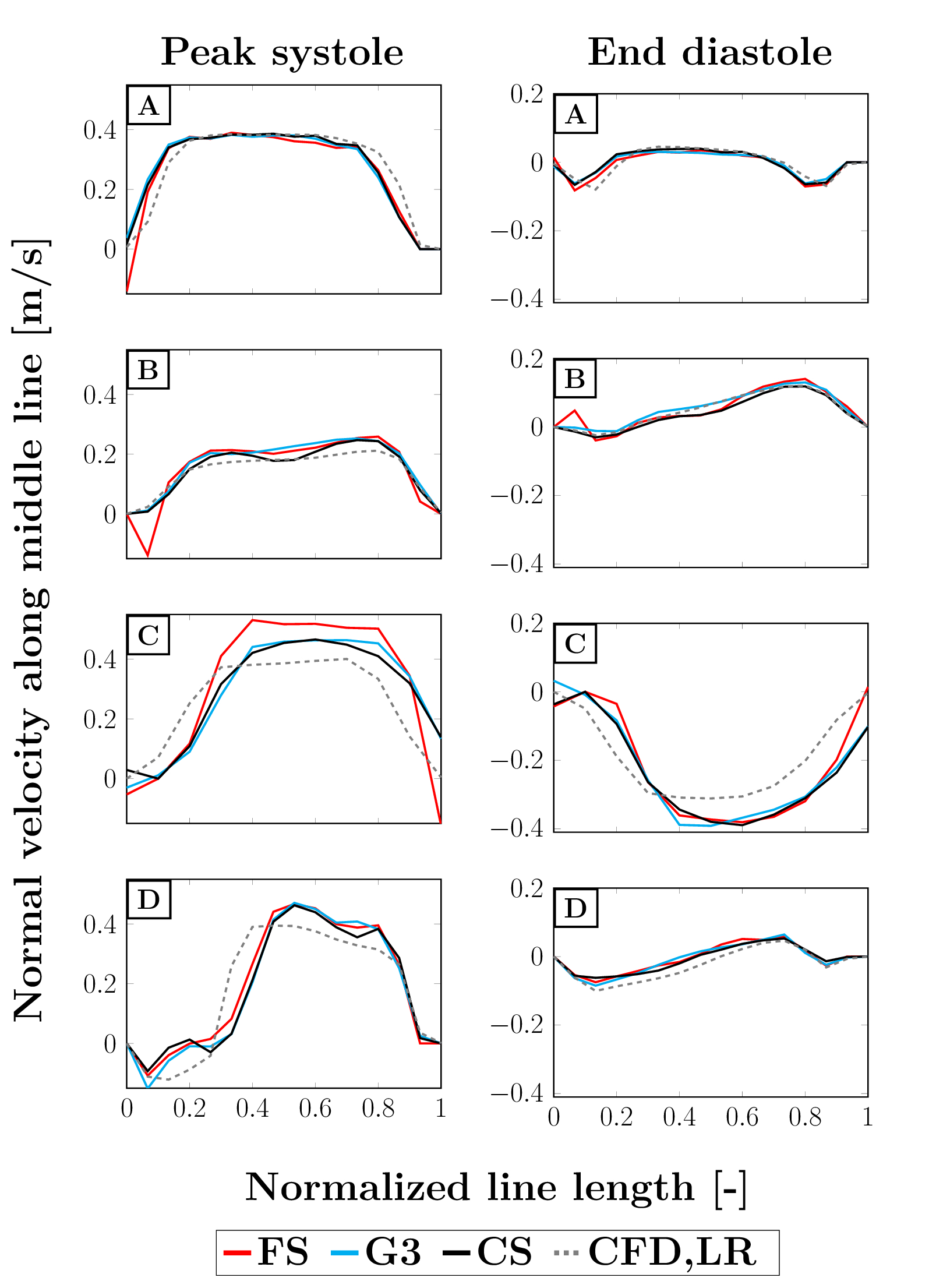
Scan times for FS, G3 and CS were 42:40, 14:40 and 5:35 min respectively. As displayed in Figure 2, the main flow structures were well captured by the different modalities at peak systole (highest flow rate at the inlet), as well as end diastole (lowest flow rate).
However, higher velocities can be observed for MRI as compared to CFD in the collateral canal and at the junction with the descending main pipe. To better appreciate the discrepancies, the normal velocity profiles are reported in Figure 3 at four locations of interest (see Figure 1). Good agreement was found between all MRI modalities, except for FS at peak systole in the collateral where higher normal velocities are recorded. Good agreement with CFD,LR was also found for low velocities. However, the values reported by CFD in the collateral and at peak diastole in the junction are lower in magnitude and the profiles appear shifted.
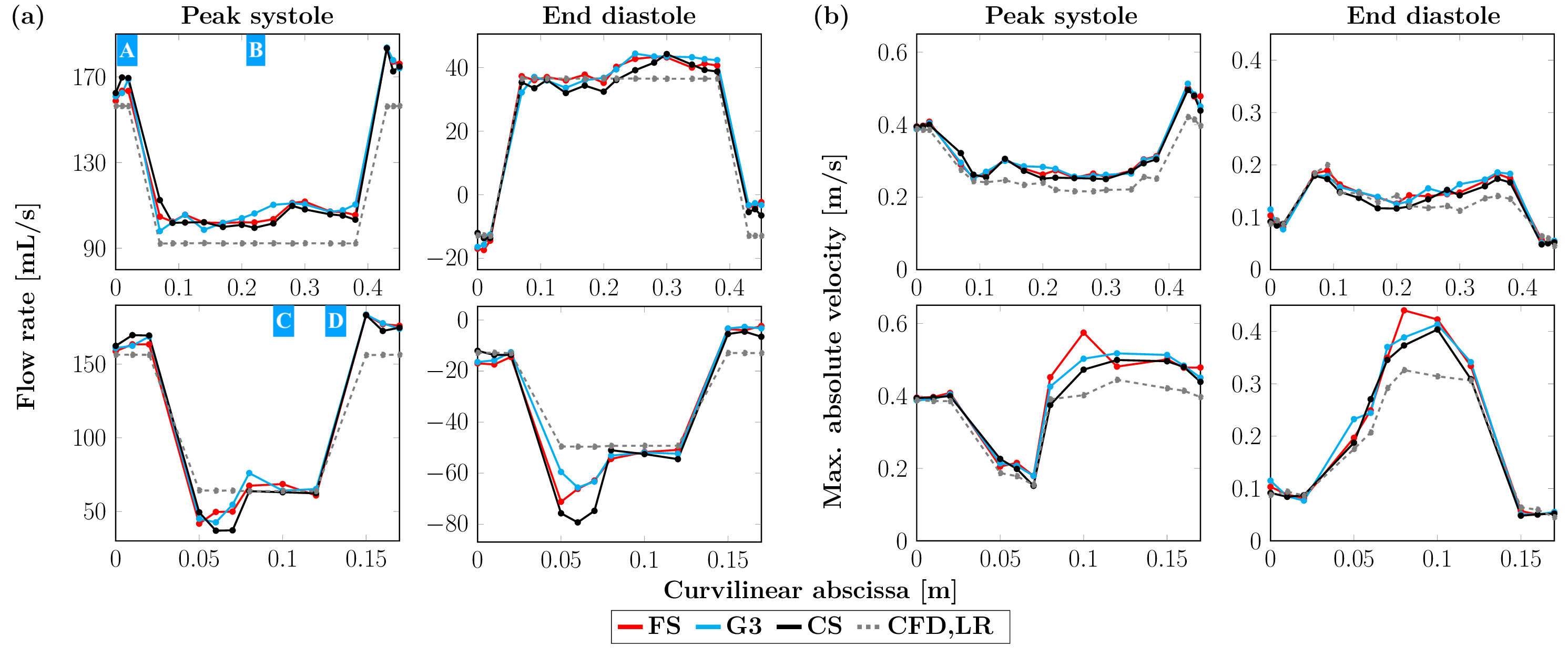
Concerning flow rates as displayed in Figure 4 (a), similar patterns were observed for the different MRI acquisitions, although the principle of mass conservation appears not to be met, especially in the aneurysm-like section and between the ascending and descending main pipes. At peak diastole, the average flow rates (in mL, reported as mean ± SD) respectively for FS, G3, CS and CFD,LR were found to be 105.2 ± 3.4, 105.6 ± 4.5, 104.0 ± 4.0 and 92.2 ± 0.1 in the upper part of the phantom and 56.4 ± 10.9, 57.9 ± 12.9, 52.1 ± 12.8 and 64.0 ± 0.2 in the collateral duct. At end diastole, the following values were reported: on the one hand 39.3 ± 2.9, 39.3 ± 4.3, 37.2 ± 3.8 and 36.5 ± 0.0, and on the other hand -59.6 ± 8.4, -57.7 ± 6.0, -64.6 ± 13.2 and -49.4 ± 0.2. The peak velocities along the same paths as the flow rates are presented in Figure 4 (b) and were computed only on voxels entirely inside the phantom volume to avoid noise due to partial volume effects. In a global manner, these velocities were equal or higher for MR acquisitions compared to the ones found for the CFD simulations, for which mass is conserved.

DISCUSSION

Velocity profiles, flow rates and peak velocities were investigated under the same flow conditions for a fully-sampled MR acquisition, as well as two acceleration techniques: GRAPPA and compressed sensing. Contrarily to what was previously observed⁴, the results were comparable for all three techniques, suggesting that compressed sensing is a suitable modality to perform fast 4D flow acquisitions. However, mass appears not to be conserved, especially in the aneurysm-like region, where highly disturbed flow patterns occur. Furthermore, the sections where the MR velocity profiles deviate from the ones simulated by the CFD correspond to locations associated with high flow velocity or acceleration. These discrepancies can most probably be related to spatial and velocity displacement artifacts⁵. MR globally overestimates the flow rates compared to CFD. Future work could include investigating more physiological flow rates waveforms, implementing post-processing methods to compensate the previously mentioned artifacts⁶ or simulating 4D flow MRI to further characterize the observed divergences⁷.

Acknowledgements

No acknowledgement found.