Introduction & Theory

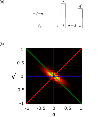
Recently, a novel technique for measuring the diffusion propagator was introduced¹. The employed diffusion encoding gradient waveform (Figure 1a) involves two independent wavenumbers, $$$q$$$ and $$$q’$$$. Sampling different lines on the $$$qq’$$$ plane as shown in Figure 1b could reveal different characteristics of diffusion. For example, the blue lines ($$$q’=0$$$ or $$$q=0$$$) depict the sequence by Laun et al.², used for diffusion pore imaging. Stejskal-Tanner measurements³ sample the $$$q’=-q$$$ line (green) and reveal the distribution of net displacements through^4,5
$$\bar{P}_\Delta(\Delta\mathbf{x})=\frac{1}{(2\pi)^d}\int\rm{d}\mathbf{q}\,e^{i\mathbf{q}\cdot\Delta\mathbf{x}}\,E(\mathbf{q})\qquad (1).$$
Here, $$$\Delta\mathbf{x}=\mathbf{x}’-\mathbf{x}$$$, where $$$\mathbf{x}$$$ and $$$\mathbf{x’}$$$ represent the positions encoded by the two pulses, respectively. The low-$$$\mathbf{q}$$$ regime of the signal is governed by
$$E(\mathbf{q})\approx\exp\left[-\left(q_x^2\langle{\Delta{x}}^2\rangle+q_y^2\langle{\Delta{y}}^2\rangle+q_z^2\langle{\Delta{z}}^2\rangle+2q_xq_y\langle{\Delta{x}}{\Delta{y}}\rangle+2q_xq_z\langle{\Delta{x}}{\Delta{z}}\rangle+2q_yq_z\langle{\Delta{y}}{\Delta{z}}\rangle\right)\right]\qquad (2).$$
More generally for the waveform in Figure 1a, a particle’s coordinates during the application of the second and third pulses ($$$\mathbf{x}$$$ and $$$\mathbf{x’}$$$) are encoded in a frame of reference whose origin is at the center-of-mass of that particle’s trajectory during the first pulse^1,6. For the case of $$$q’=q$$$, we introduce $$$\mathbf{Q}=2\mathbf{q}$$$ and define the “mean position” as $$$\mathbf{\bar{x}}=(\mathbf{x}+\mathbf{x’})/2$$$.
The signal $$$E(\mathbf{Q})$$$ acquired through this scheme can then be used to estimate the mean position distribution through the following Fourier Transform:
$$\bar{P}_\Delta(\mathbf{\bar{x}})=\frac{1}{(2\pi)^d}\int\rm{d}\mathbf{Q}\,e^{i\mathbf{Q}\cdot\mathbf{\bar{x}}}\,E(\mathbf{Q})\qquad (3).$$
The low-$$$\mathbf{Q}$$$ behavior of the signal is then,
$$E(\mathbf{Q})\approx\exp\left[-\left(Q_x^2\langle{\bar{x}}^2\rangle+Q_y^2\langle{\bar{y}}^2\rangle+Q_z^2\langle{\bar{z}}^2\rangle+2Q_xQ_y\langle{\bar{x}}{\bar{y}}\rangle+2Q_xQ_z\langle{\bar{x}}{\bar{z}}\rangle+2Q_yQ_z\langle {\bar{y}}{\bar{z}}\rangle\right)\right]\qquad (4).$$
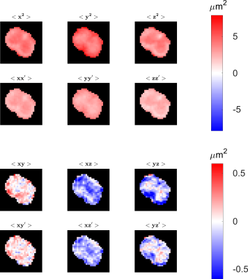
Using Equation 4, the position-dependent quantities can be cast as a squared mean-position tensor. Similarly, from Equation 2, a squared displacement tensor can be obtained. Simple algebraic manipulations of these tensors’ components reveal 12 unique quantities, six of which are “static” (at the same point in time) correlations of particle positions: $$$\langle{x^2}\rangle,\langle{y^2}\rangle,\langle{z^2}\rangle,\langle{xy}\rangle,\langle{xz}\rangle,\langle{yz}\rangle$$$. The remaining quantities for “dynamic” (at different points in time) correlations are: $$$\langle{xx'}\rangle,\langle{yy'}\rangle,\langle{zz'}\rangle,\langle{xy'}\rangle,\langle{xz'}\rangle,\langle{yz'}\rangle$$$.
Here, we present the very first application of the above-introduced techniques on biological tissue.

Methods

The pulse sequence presented in Figure 2 was implemented on a benchtop MRI scanner (Pure Devices GmbH, Germany). This pulse sequence differs from a previous embodiment of the technique⁶ in that only the first gradient of the effective waveform of Figure 1a was implemented as a bipolar pulse pair in an effort to approach the narrow pulse regime.
The investigated sample was an excised mouse spinal cord (obtained following national and local ethical guidelines). All imaging was performed with a matrix size of $$$48\times48$$$ and an in-plane voxel size of approximately $$$0.1\times0.1 mm^2$$$.
For the first experiment, all diffusion gradients were applied along a single direction, perpendicular to the direction of the fibers in white matter. Two datasets were acquired, respectively, with $$$q’=q$$$ and $$$q’=-q$$$. The values of q applied in this study ranged from $$$-0.8 rad/\mu m$$$ to $$$+0.8 rad/\mu m$$$ with 15 regularly-spaced samples. Each acquisition was repeated 20 times, averaged, and filtered with a simple Gaussian filter.
The second experiment involved a two-shell acquisition with 6 and 21 directions applied at low and high b-values, respectively. Two datasets were acquired, the first setting $$$q’=q$$$ and the second with $$$q’=-q$$$. The values of q were set to obtain approximately the same b-value in both cases. Each acquisition was repeated 25 times, averaged, and filtered with a simple Gaussian filter.
Complex data acquired from the scanner were used in the reconstruction pipeline for the first experiment, which involved the estimation of the mean position distribution $$$\bar{P}_\Delta(\bar x)$$$, and the displacement distribution $$$\bar{P}_\Delta(\Delta\mathbf{x})$$$^4,7.
For the second experiment, magnitude-valued data from both acquisitions were processed to estimate the squared displacement and squared mean-position tensor components following Equations 2 and 4, respectively.
All computations were performed using MATLAB (Mathworks Inc., Natick, MA, USA).

Results

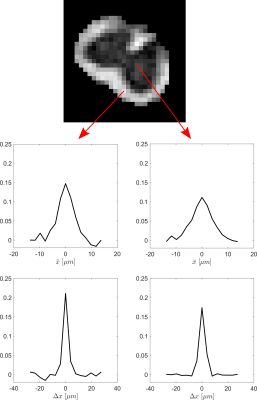
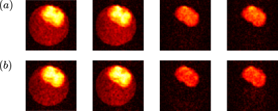
The real part of the estimated displacement distribution and mean position distribution for voxels corresponding to, respectively, white matter and gray matter are presented in Figure 3.
Four of the twenty-seven images corresponding to the spinal cord sample acquired in the second experiment for each acquisition, i.e., with $$$q’=-q$$$ and $$$q’=q$$$, are presented in Figure 4.
The 12 unique component images corresponding to both static and dynamic correlations of positions obtained from the squared displacement and squared mean-position tensors are presented in Figure 5.

Discussion & Conclusion

In this study, we introduced a new method for determining the mean-position distributions. It should be kept in mind that the mean-position is defined in a frame of reference whose origin coincides with the average position of the particles during the application of a long pulse. Because of this, the distributions have finite extent much like the displacement distributions revealed by the Stejskal-Tanner sequence, which is the standard method for investigating compartmentalization in biological specimens⁵. There are important differences in the two distributions however, as illustrated by our results from the spinal cord specimen.
The low diffusion sensitivity regime of the signal is also studied here. The required sampling resembles that for diffusion tensor imaging⁸ and complements it by revealing the second moments of the mean positions. Synergistic application of the two techniques unraveled dynamic moments from static ones providing various contrasts within the excised mouse spinal cord.
In conclusion, a sophisticated framework involving new data acquisition and analysis schemes is introduced. Its feasibility is illustrated on a benchtop MRI scanner. The technique complements the existing methods in a meaningful way and could be instrumental in investigating numerous challenges that demand novel characterization methods.

Acknowledgements

We are grateful to Anders Eklund for his support in the acquisition of the MR scanner, and to Walker Jackson for providing the sample investigated in this study.