Introduction

Cerebral intravoxel incoherent motion (IVIM) is a diffusion-weighted MR imaging technique that has the potential to simultaneously measure the parenchymal diffusivity and microvascular perfusion¹. Recently, it was shown that a third, intermediate, IVIM-component can be extracted from the IVIM signal². This additional component is thought to be related to the interstitial fluid (ISF) in the extracellular or perivascular spaces³.

Estimating the intermediate IVIM component can be challenging, since spectral decomposition using the non-negative least squares (NNLS) is an ill-posed technique with strong dependence on the number of samples (i.e. acquired b-values) and SNR. Since acquisition time limits the total number of acquired b-values, it is important to know which b-values are essential to be acquired. Therefore, in this study we will assess an optimal b-value sampling strategy for estimating the intermediate component. The optimal sampling will be derived using a genetic algorithm⁴ and simulated data. Subsequently, the performance of the optimal sampling will be compared to a linear and logarithm sampling using simulations and in vivo data.

Methods

Numerical simulations
To evaluate the optimal b-value sampling scheme, ground-truth IVIM signals were synthesized using,
$$S(b)=S_0[(1-f_{int}-f_{mv})e^{-bD_{par}}+f_{int}e^{-bD_{int}}+f_{mv}e^{-bD_{mv}}]+\varepsilon_{b}$$
where, $$$f_{int}$$$ and $$$f_{mv}$$$ are amplitude fractions of the intermediate and microvascular components. $$$D_{par}$$$, $$$D_{int}$$$ and $$$D_{mv}$$$ are the diffusivities for the parenchymal, intermediate and microvascular components.

Decay curves were synthesised with diffusivity values randomly sampled from a uniform distribution with the following ranges, $$$.1\cdot10^{-3}\leq D_{par}<1.5\cdot10^{-3}mm^2/s$$$, $$$1.5\cdot10^{-3}\leq D_{int}<4.0\cdot10^{-3}mm^2/s$$$ and $$$4.0\cdot10^{-3}\leq D_{mv}\leq4.0\cdot10^{-3}mm^2/s$$$. Similarly, the amplitude fractions were randomly sampled from a uniform distribution, where $$$.0\leq f_{mv}\leq .1$$$ and $$$.0\leq f_{int}\leq.3$$$. To simulate the effect of noise, 100.000 Gaussian noise realizations were performed with an SNR of 100 at b=0 s/mm².

MRI acquisition
A single subject (67y, male) underwent high-field MRI (7T Magnetom, Siemens Healthcare, Erlangen, Germany). IVIM images were acquired using a multi-shot spin-echo echo-planar-imaging sequence (TR/TE=22800/57.6ms; resolution=1.5x1.5mm, thickness=3.5mm, acceleration-factor=2, acquistion time=49 minutes), after cerebrospinal fluid suppression (TI=2330ms). 101 diffusion sensitive b-values were acquired, ranging from 0 to 1000 with increments of 10 s/mm². The IVIM images were corrected for head displacements.

IVIM analysis
The IVIM data is analysed with the NNLS algorithm, using a basis set of 200 logarithmically spaced functions. From the obtained spectrum, the $$$f_{int}$$$ is calculated as the ratio of the intermediate components ($$$D_{int}$$$) to the amplitude of all components. For the in vivo data, the resulting amplitude fractions were subsequently corrected for T1 and T2 relaxation effects².

Genetic Algorithm
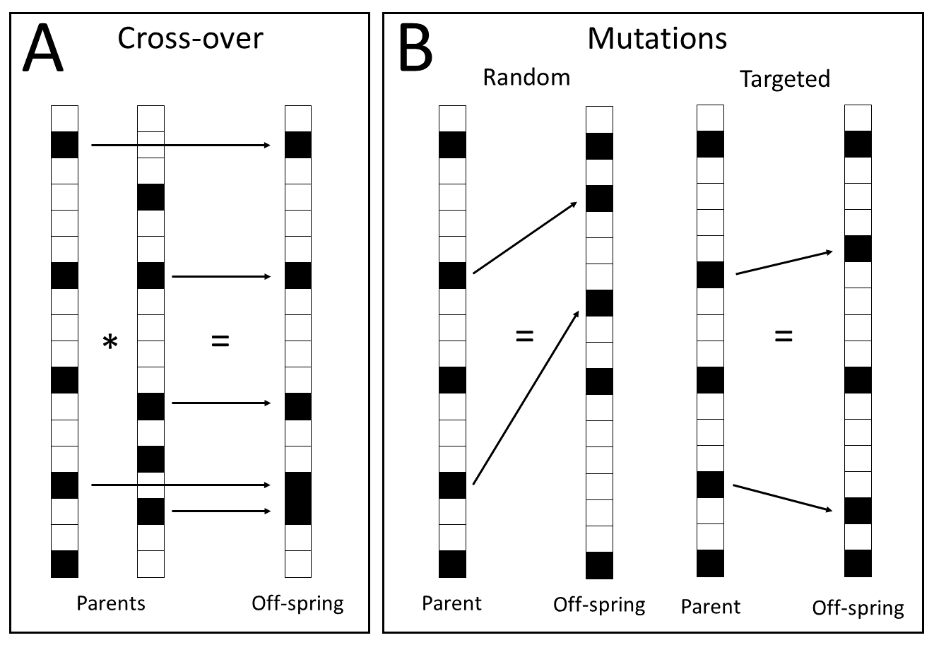
First, a random population (i.e., first generation) will be initialized as 100 binary vectors of length 101 with 15 non-zero elements (b-values ranging from 0 up to 1000 s/mm² with increments of 10 s/mm2). Second, the performance of each b-value sampling scheme will be assessed by the root mean squared error (RMSE) of the estimation of $$$f_{int}$$$,
$$FF=\sqrt{\frac{1}{N}\Sigma_{i=1}^{N}{\Big(\widehat{f}_{int} -f_{int}\Big)^2}}$$
where $$$FF$$$ is the fitness function, $$$N$$$ is the number of noise realisations, $$$\widehat{f}_{int}$$$ is the ground-truth and $$$f_{int}$$$ is the estimated amplitude fraction of the intermediate component. The 20 samplings with the best performance, i.e. parents, will be kept for the next generation, while the other 80 will be replaced by 40 new sampling schemes obtained using cross-over and 40 using mutations (Figure 1). This process is repeated up to the 250^th generation. The only constraint is that the b-value samplings must include b=0 s/mm², since this is required for normalizing the IVIM signal.

Evaluation
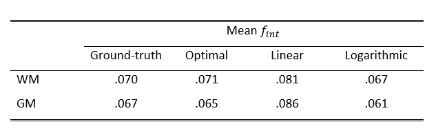
The performance of the optimal b-value sampling strategy was compared to a linear and logarithmic sampling in terms of the RMSE of $$$f_{int}$$$. For the in vivo data, a ground-truth is calculated as the mean $$$f_{int}$$$ of the white matter (WM) as well as the gray matter (GM) using a voxel-wise fit where all 101 b-values are included. Subsequently, the mean $$$f_{int}$$$ of the optimal sampling is compared to the ground-truth, as well as to the linear and logarithmic b-value samplings.

Results

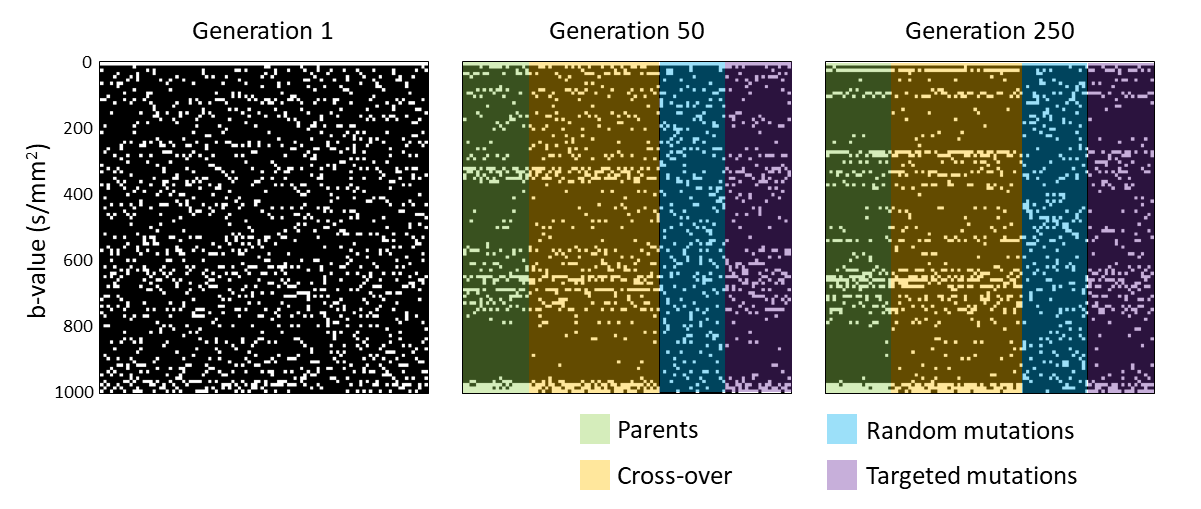
The evolution of the population (i.e. the b-value sampling schemes) over several generations is shown in Figure 2. The optimal b-value sampling is found to be; 0,20,100,270,280,370,540,650,660,710,720,790,980,990,1000 s/mm². For the simulated data, the optimal b-value sampling strategy was found to be at least 1.24 times more accurate compared to linear and logarithmic sampling in terms of RMSE (optimal: .29 vs reference: .36 vs linear: .36).
For the in vivo data, the optimal sampling strategy resulted in a mean $$$f_{int}$$$ that very close to the ground-truth for both WM and GM. Moreover, the mean $$$f_{int}$$$ of the optimal sampling best approximates the ground-truth compared to the linear and logarithmic sampling (Table 1).
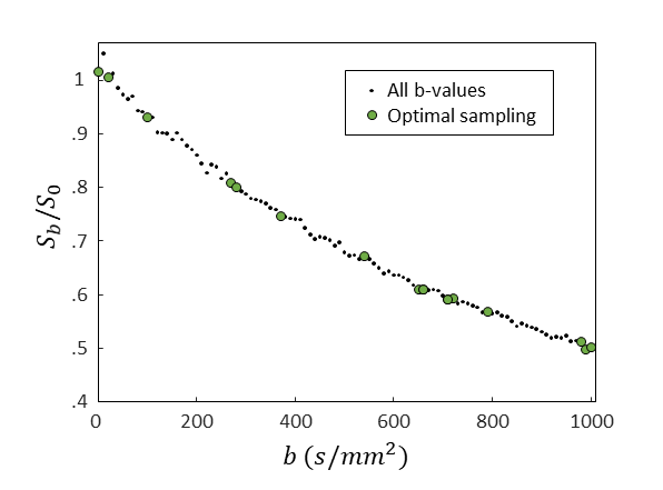
An IVIM decay curve of the in vivo data, including the optimal sampling, is shown in Figure 3.

Discussion & Conclusion

This study presents an optimal b-value sampling for estimating $$$f_{int}$$$. The optimal sampling was shown to outperform linear and logarithmic sampling strategies, for both simulations and in vivo data. From previous work on mono-exponential decaying functions⁵, we expect that the b-value range corresponding to $$$D_{int}\cdot b\approx1.3$$$ would be especially beneficial for estimating $$$f_{int}$$$. Since the intermediate range is $$$1.5\cdot10^{-3}\leq D_{int}<4.0\cdot10^{-3}mm^2/s$$$, this would correspond to the range b=325 to 867 s/mm². Indeed, our results show that this b-value range is important, since half of the ‘optimal’ b-values span this range.

Acknowledgements

No acknowledgement found.