INTRODUCTION

Magnetic resonance spectroscopy (MRS) and spectroscopic imaging (MRSI) can provide information about local metabolite concentrations in living tissues non-invasively, but its utility can be limited by a low signal-to-noise ratio (SNR) in practice. Averaging multiple coherent repetitions increases the SNR, but at the cost of time-consuming acquisition. Use of MRSI data denoising may result in a higher SNR by utilizing the low-rank structures of the MRSI data without the need of the lengthy multiple scan acquisition¹. Low-rank approximation approaches can be used for denoising data without relying on MR-theoretical prior knowledge^1–3. However, most existing denoising methods rely upon linear complexity reduction of each time/frequency-domain vector of an MRSI data set, which results in information loss⁴. Deep learning (DL) has been used to incorporate learned non-linear models based on prior knowledge to constrained MRSI data reconstruction⁴.
This work proposes an unsupervised DL approach applying a data-driven non-linear model and low-dimensional representation of MRS(I) data for MRS(I) signal denoising.

METHODS

The MRSI data of a phantom containing milk cream (~30% fat) were acquired by bipolar multi-gradient-echo sequences in two measurements with the following parameters common for the both: spatial acquisition matrix = 128x128 voxels; voxel size = 352 x 320 x 1000 µm³; bandwidth = 5580 Hz/voxel; TR = 1300 ms; FA = 30°; NA = 2. In each measurement 1024 echo images were acquired, with echo spacing of 500 µs with the first echoes at 714 µs and 964 ms, respectively. Phase correction of bipolar readout gradients was applied⁵. Data from both measurements were interlaced so that 250 ms echo spacing was ensured.
A simulated (numerical) phantom contains 128x128 signals, each with two Lorentzian components located at 4.7 ppm and at 1.2 ppm, with linewidths in the range of [45, 50] and amplitudes in the ranges of [0.5, 1] and [0.05, 0.1], respectively. Amplitudes and linewidths were drawn randomly and independently from uniform distributions.
The SNR of signals (time origin magnitude to noise standard deviation expressed in the logarithmic decibel scale) was set in the range of 10.5 to 15.5 dB by introducing random complex Gaussian noise.
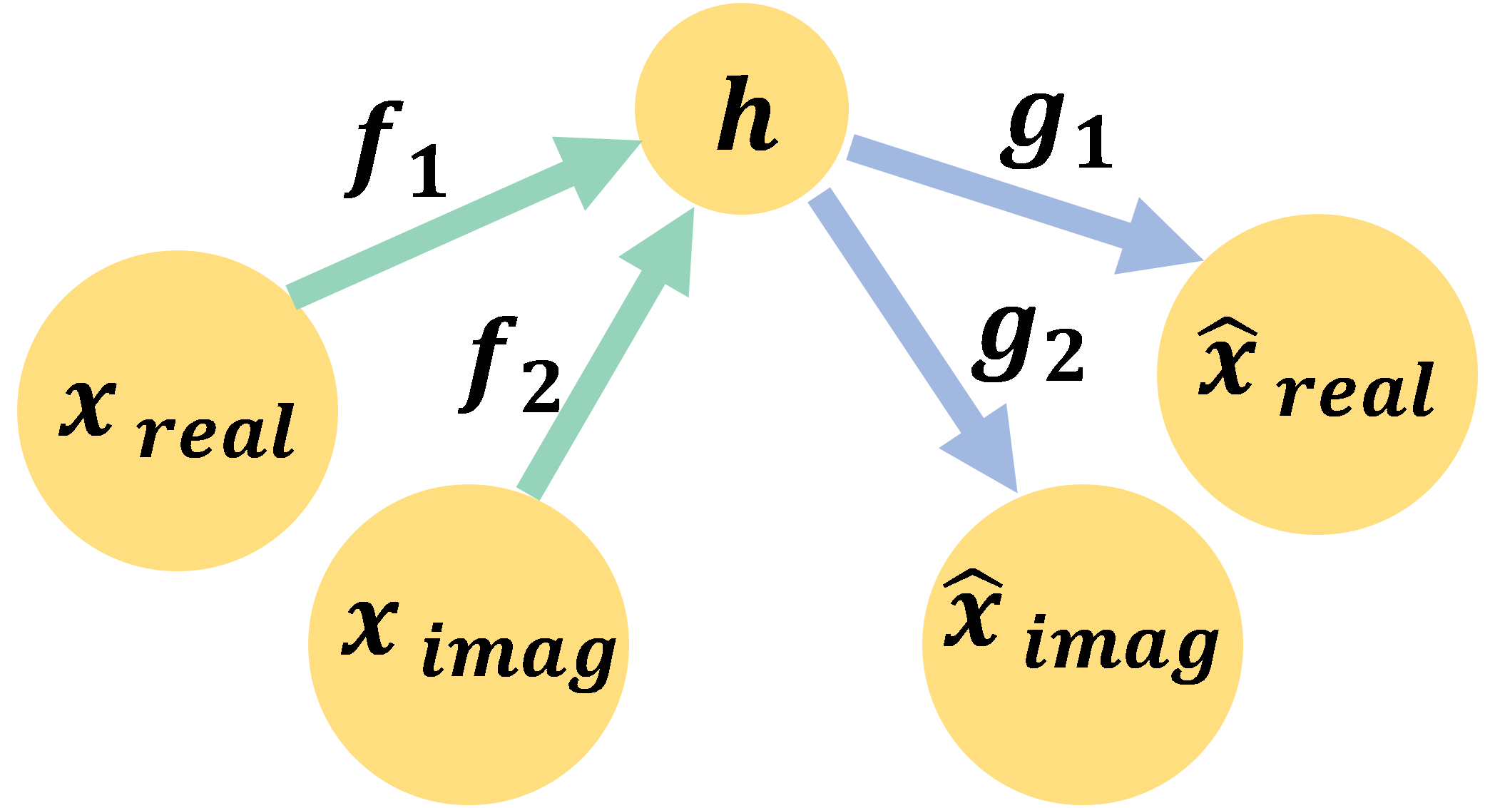
A deep autoencoder (AE) is able to learn an accurate and robust low-dimensional model for data. Figure 1 illustrates the architecture of the implemented AE. The AE is composed of sequential layers of fully connected and rectifier linear unit layers. The AE is trained by minimizing the dissimilarity between the input and the output. The AE learns latent spaces with a low effective dimension by introducing several additional linear layers between the encoder and the decoder⁶.
Using the following formulation, the trained AE is incorporated into the denoising process:
$$\begin{equation} \underset{h}{\mathrm{argmin}}\;{|x-g(h)| + \lambda \sum_{i=0}^{16}{|h_{i}|}} \end{equation}$$
where the $$${x}$$$ is the noisy signal, $$${\lambda}$$$ is a tuning parameter, $$${g}$$$ is the learned decoder function, and $$${h}$$$ is a non-negative vector (i.e. $$${h_{i}\geq {0} \, {∀i}}$$$) of the representation in latent space. The first term enforces data consistency between the noisy input and the output of the decoder. The second term involves a penalty on the latent layer whose strength is controlled by $$${\lambda}$$$. The above equation can be viewed as non-linear programming (NLP) process, which can be solved by direct search methods like Nelder–Mead⁷.
All steps were run on a computer with a dual EPYC 7742 processor and one graphics processing unit (NVIDIA A100). The AE was implemented using the PyTorch framework^8,9. All training was performed using the mean-squared error loss and an Adam optimizer¹⁰ with a batch size of 32, learning rate 1e-5, and 150 epochs.
The network was trained using signals from all voxels of the MRSI data that should be denoised with the network.

RESULTS

Figure 2 shows a set of results achieved by our method from the real phantom.
Figure 3 shows the effect of the tuning parameter on denoising performance.
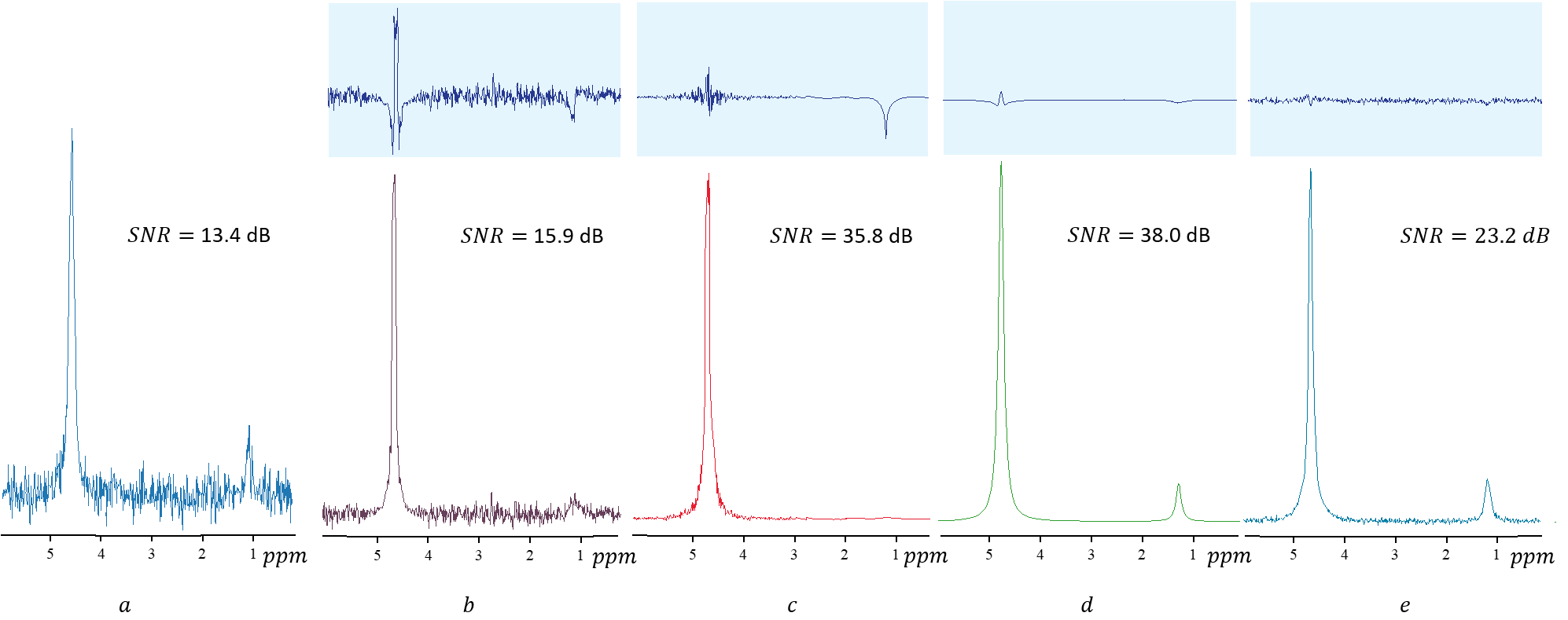
A comparison between the denoising results from our proposed method, a discrete wavelet transform¹¹, LORA^1,2, and the Truncated singular value decomposition (TSVD)² is shown in Figure 4.
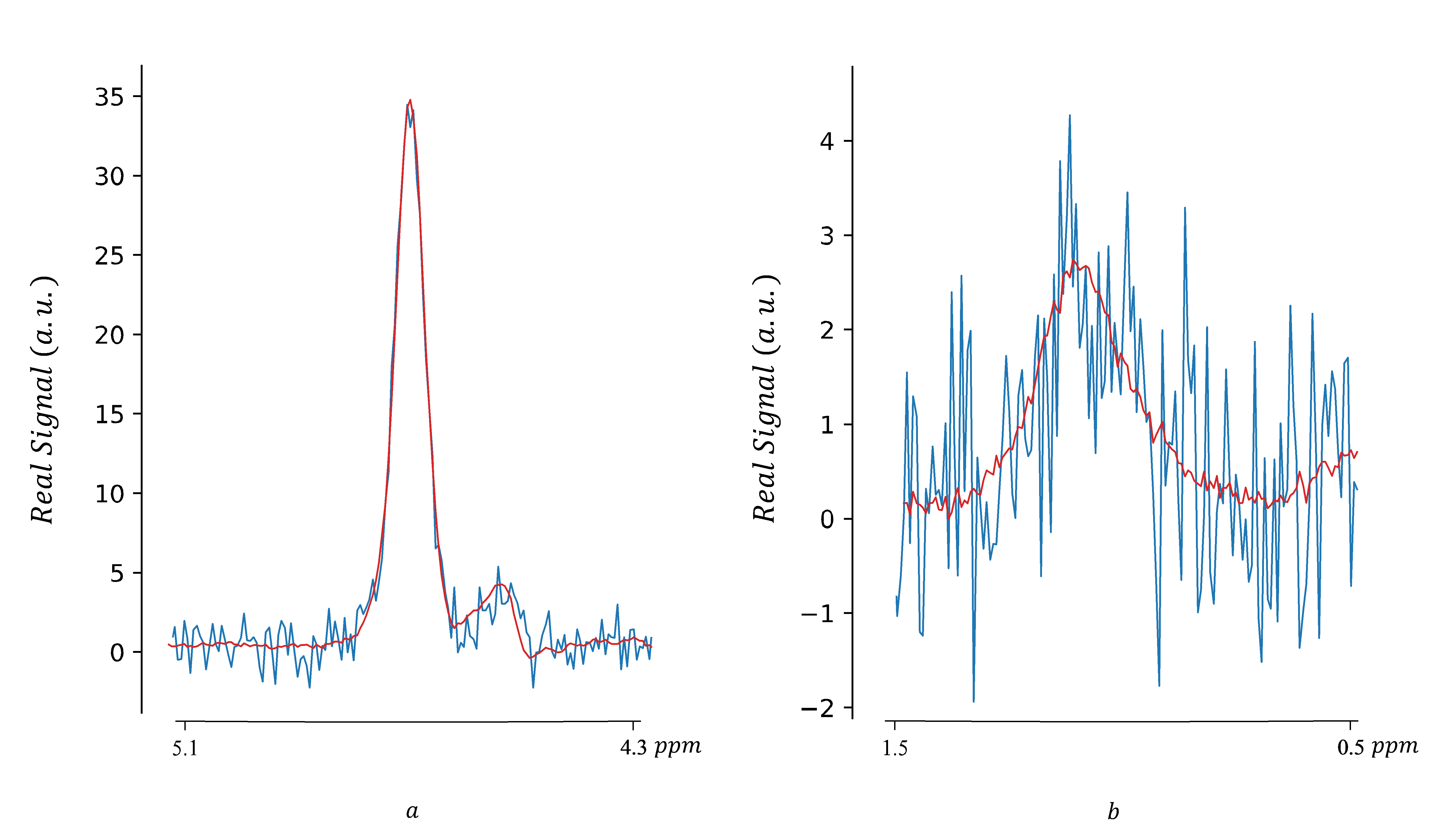
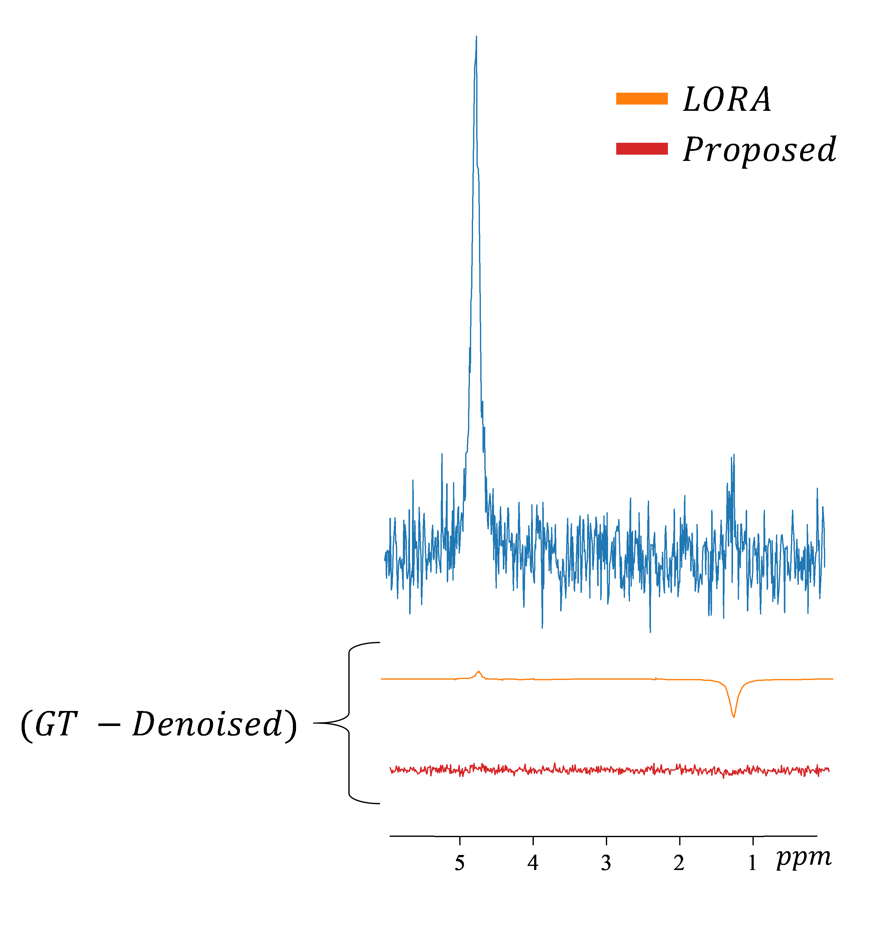
Figure 5 shows the comparison between denoising performance using LORA and our proposed method for a signal with a relatively low concentration at the 1.2 ppm peak.

DISCUSSION

From visual inspection, the proposed method outperforms methods using TSVD and the discrete wavelet transform. While the proposed method is less effective than LORA algorithm in terms of increasing SNR, it might be more robust in low concentration component denoising. In general, SNR might not be the only indicator of the performance of a denoiser².
The AE could be trained with clean data¹² synthesized with lineshape modeling or by quantum mechanical simulation. However, using MR-theoretical prior knowledge might bias the result in the subsequent processes.
The attractiveness of the proposed method is that no MR-theoretical prior knowledge is enforced.
Like estimating the rank threshold, finding the best value for the tuning parameter is challenging in practice.

CONCLUSION

The proposed method can achieve results comparable with other techniques while preserving the information of low concentration components. Deep learning data denoising for MRSI might result in a faster acquisition, which is vital for MRSI clinical application. However, additional studies should be done for more complex MR signals with overlapping peaks.

Acknowledgements

This project has received funding from the European Union's Horizon 2020 research and innovation program under the Marie Skłodowska-Curie grant agreement No 813120.

References

1. Nguyen HM, Peng X, Do MN, et al. Denoising MR spectroscopic imaging data with low-rank approximations. IEEE Trans Biomed Eng 2013;60:78-89.

2. Clarke WT, Chiew M. Uncertainty in denoising of MRSI using low-rank methods. Magn Reson Med 2021:1-15.

3. Yin M, Smith RS. On Low-Rank Hankel Matrix Denoising. 2020.

4. Lam F, Li Y, Peng X. Constrained Magnetic Resonance Spectroscopic Imaging by Learning Nonlinear Low-Dimensional Models. IEEE Trans Med Imaging 2020;39:545-555.

5. Eckstein K, Dymerska B, Bachrata B, et al. Computationally Efficient Combination of Multi-channel Phase Data From Multi-echo Acquisitions (ASPIRE). Magn Reson Med 2018;79:2996-3006.

6. Jing L, Zbontar J, Lecun Y. Implicit Rank-Minimizing Autoencoder. 2020.

7. Gao F, Han L. Implementing the Nelder-Mead simplex algorithm with adaptive parameters. Comput Optim Appl 2010 511 2010;51:259-277.

8. Paszke A, Gross S, Massa F, et al. PyTorch: An imperative style, high-performance deep learning library. Adv Neural Inf Process Syst 2019;32.

9. WA Falcon et al. No Title. GitHub Note https//github.com/PyTorchLightning/pytorch-lightning 2019.

10. Kingma DP, Ba JL. Adam: A method for stochastic optimization. In: 3rd International Conference on Learning Representations. International Conference on Learning Representations, ICLR, 2015. https://arxiv.org/abs/1412.6980v9. Accessed April 29, 2021.

11. MProx/Wavelet-denoising: A script to use the PyWavelet library to perform denoising on a signal using a multi-level signal decomposition using a discrete wavelet transform. https://github.com/MProx/Wavelet-denoising. Accessed October 28, 2021.

12. Lehtinen J, Munkberg J, Hasselgren J, et al. Noise2Noise: Learning image restoration without clean data. 35th Int Conf Mach Learn ICML 2018 2018;7:4620-4631.