0842

An untrained deep learning method with model-based regularization for reconstructing dynamic MR images from retrospectively accelerated data

Kalina P Slavkova¹, Julie C DiCarlo^2,3, Viraj Wadhwa⁴, Thomas E Yankeelov^2,3,5,6,7, and Jonathan I Tamir^2,4,6
¹Department of Physics, The University of Texas at Austin, Austin, TX, United States, ²Oden Institute for Computational Engineering and Sciences, The University of Texas at Austin, Austin, TX, United States, ³Livestrong Cancer Institutes, The University of Texas at Austin, Austin, TX, United States, ⁴Department of Electrical and Computer Engineering, The University of Texas at Austin, Austin, TX, United States, ⁵Department of Biomedical Engineering, The University of Texas at Austin, Austin, TX, United States, ⁶Department of Diagnostic Medicine, The University of Texas at Austin, Austin, TX, United States, ⁷Department of Oncology, The University of Texas at Austin, Austin, TX, United States

Synopsis

Acquiring high-resolution MRI data for tissue parameter mapping for quantitative imaging requires additional scan time. As a proof-of-principle, we evaluated the ability of the ConvDecoder architecture regularized with a physical model to reconstruct accelerated variable-flip angle MRI data of the brain for T₁-mapping. The performance of our method was compared to non-regularized ConvDecoder, low rank reconstruction, and compressed sensing. Our results suggest that ConvDecoder with physics-based regularization may provide a stopping condition for training that is not dependent on the ground truth data while improving parameter mapping at higher accelerations.

Introduction

T₁-mapping by the variable-flip angle (VFA) method requires the acquisition of T₁-weighted MRI data at a series of different flip angles, which are then fit to the fast spoiled gradient echo (FSPGR) model to estimate the T₁ values of the tissues at each voxel¹. This parameter mapping is necessary in some quantitative imaging schemes^2,3. Ideally, shortening the VFA scan would optimize data acquisition while maintaining spatial resolution for improved quantitative imaging. While untrained methods^4-7 have shown promise toward this goal without requiring training data^8-10, they often do not incorporate known physics. We previously demonstrated the utility of the untrained ConvDecoder (CD)⁴ method with a FSPGR-based regularization term (CD+r) for reconstructing images from simulated accelerated VFA data¹¹. Here, we apply the CD+r¹¹ method to reconstruct images from retrospectively accelerated raw VFA data collected from three healthy subjects. We compare the image reconstruction quality and T₁ map output of the fully-sampled VFA data to the output of the retrospectively accelerated VFA data reconstructed with CD+r, CD, parallel imaging with low rank regularization¹² (LR), and compressed sensing¹³ (L1). We show that CD+r provides a stopping condition for training, which is promising for prospective accelerated data acquisition with no fully-sampled ground truth for determining the optimal reconstruction.

Methods

VFA acquisition: Healthy subjects (N=3) were scanned on a 3T MAGNETOM Vida scanner (Siemens, Munich, Germany) equipped with a 32-channel coil array (Siemens, Munich, Germany) under IRB approval and with informed consent. The fully-sampled VFA data were collected using a 50-minute FSPGR sequence with an acquisition matrix of 224×224, TR/TE = 6.10/2.75 ms, and flip angles θ$$$\in$$${4°,6°,8°,10°,12°,14°,16°,18°,20°}. A representative dynamic slice from each dataset was selected for analysis.
Simulated data: We evaluated the case of no VFA model error using simulated data. All three fully-sampled VFA anatomical images were fit to the FSPGR model through dictionary matching¹⁴ with a dictionary, D(T₁,θ), created from 2,000 T₁ values linearly spaced between 50 ms and 4000 ms. Noise was added to each fit based on the computed SNR of each dataset.
Retrospective acceleration: The fully-sampled raw and simulated data were each retrospectively under-sampled at each θ using unique 2D Poisson disk sampling masks (M) with fully-sampled auto-calibration regions implemented in BART¹⁵. We chose acceleration factors of R$$$\in$$${8,12,18}, corresponding to scan durations of {6.25, 4.17, 2.78} minutes.
ConvDecoder reconstruction: The MRI forward operator is $$$A=M･F･S$$$, where F is the discrete Fourier transform operator and S contains coil sensitivities estimated using ESPIRiT¹⁶. Using A, the VFA data are represented as y=Ax, where y contains accelerated k-space measurements and $$$x$$$ are the corresponding VFA anatomical images.
The CD network parameterized by weights (w) was implemented in Python with eight layers, 256 latent channels, and an input seed of size 64 and optimized using DeepInPy¹⁷. The cost function for training CD (G(w)) over w is defined as follows: $$L(G(w))=\min_w||y - AG(w)||^2_2+\mu||G(w)-\widehat{x}||^2_2,$$ $$\widehat{x}(T_1,\theta)=arg\max_{T_1}⁡(|G(z)|∙D(T_1,θ))$$
Here, μ is the regularization parameter (0 for non-regularized CD); and $$$\widehat{x}$$$ is the FSPGR model output. The model, $$$\widehat{x}$$$, was updated at an empirically chosen frequency of five epochs through alternating minimization¹⁸. Training was performed with DeepInPy for 10,000 steps with step size $$$δ=0.01$$$. For CD+r, four experiments were conducted with $$$\mu\in\left\{0.05,0.10,0.50,1.0\right\}$$$, where the regularization loss was retrospectively smoothed with the Savitzky-Golay¹⁹ method. The images saved at the closest available step to the argmin of the regularization loss were selected for analysis.
Baseline reconstruction: The raw and simulated retrospectively under-sampled k-space data for each R value were reconstructed with LR and L1 using BART. The resultant images were fit to the FSPGR model to arrive at corresponding T₁ maps.
Statistical analysis: The normalized root mean square error (NRMSE), concordance correlation coefficient (CCC)²⁰, and structural similarity index (SSIM)²¹ between the ground truth and reconstruction-based outputs were evaluated to assess the performance of our proposed framework.

Results

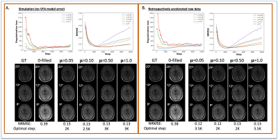
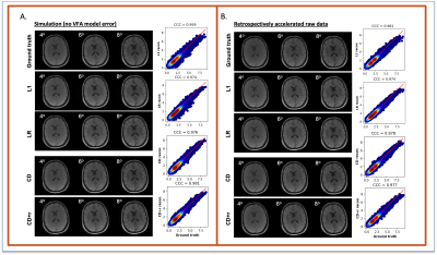
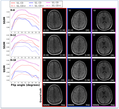
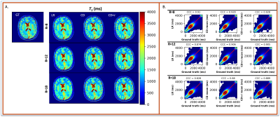
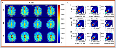
The reconstructions in Figure 1 for simulation (F1A) and experiment (F2B) at R=12 for one subject show NRMSEs within 1% of each other across all four μ’s. While this suggests a robustness under changes in μ, the regularization loss reveals earlier stopping for smaller μ’s. Taking the same subject and μ=0.10, Figure 2 shows that LR, CD, and CD+r perform similarly in recovering anatomical details in both model-free (F2A) and experimental (F2B) cases with similar CCCs. CD and CD+r show robust performance in Figure 3 across subjects at different R values in terms of SSIM. The advantage of CD+r is clear for T₁ mapping across R values and subjects in Figures 4 and 5, respectively. CD and CD+r show more anatomical details than LR, corroborated by higher CCC values, with the advantage of CD+r being the stopping condition not dependent on ground truth data.

Discussion and Conclusion

In this work, we demonstrated the utility of the stopping condition provided by CD+r. Our method yielded lower NRMSE overall in later training steps (F1A,B) and showed similar performance to the CD output with the lowest NRMSE (F3). At R=12 (4 min. acquisition), CD+r consistently yielded CCC>=0.9 in T₁ maps across subjects. Ongoing investigations include real-time minimization of the regularization loss for prospective early stopping, reconstruction of prospectively accelerated VFA data, and application to other accelerated MRI sequences with corresponding models for regularization.

Acknowledgements

We thank the National Institutes of Health for funding through NCI U01CA142565, U01CA174706, U01CA253540, U24 CA226110, and R01CA240589. We thank the American Cancer Society for support through RSG-18-006-01-CCE and the Cancer Prevention and Research Institute of Texas for support through CPRIT RR160005. We are also thankful for an AWS Machine Learning Research Award. T.E.Y is a CPRIT Scholar in Cancer Research.

References

[1] Wang HZ, Riederer SJ, Lee JN. Optimizing the precision in T1 relaxation estimation using limited flip angles. Magn Reson Med. 1987;5(5):399-416. PMID: 3431401.

[2] Yankeelov TE, Gore JC. Dynamic Contrast Enhanced Magnetic Resonance Imaging in Oncology: Theory, Data Acquisition, Analysis, and Examples. Curr Med Imaging Review. 2009;3(2): 91-107.

[3] Sorace AG, Partridge SC, Li X, Virostko J, Barnes SL, Hippe DS, Huang W, Yankeelov TE. Distinguishing benign and malignant breast tumors: preliminary comparison of kinetic modeling approaches using multi-institutional dynamic contrast-enhanced MRI data from the International Breast MR Consortium 6883 trial. Journal of Medical Imaging. 2018;5(1):011019.

[4] Darestani M, & Heckel R. (2020). Accelerated MRI with Un-trained Neural Networks. arXiv preprint arXiv:2007.02471v3.

[5] Van Veen D, Jalal A, Soltanolkotabi M, Price E, Vishwanath S, Dimakis AG. Compressed sensing with deep image prior and learned regularization. arXiv preprint. 2018; arXiv:1806.06438.

[6] Ulyanov D, Vedaldi A, & Lempiitsky V. Deep Image Prior. arXiv preprint. 2017; arXiv: 1711.10925.

[7] Heckel R, Hand P. Deep Decoder: Concise Image Representations from Untrained Non-convolutional Networks. arXiv preprint. 2018. arXiv:1810.03982.

[8] Aggarwal HK, Mani MP, Jacob M. MoDL: Model-based deep learning architecture for inverse problems. IEEE transactions on medical imaging. 2018;38(2):394-405.

[9] Liu F, Kijowski R, El Fakhri G, Feng L. Magnetic resonance parameter mapping using model-guided self-supervised deep learning. Magnetic Resonance in Medicine. 2021; 85(6):3211-3226

[10] Hammernik K, Klatzer T, Kobler E, Recht MP, Sodickson DK, Pock T, Knoll F. Learning a variational network for reconstruction of accelerated MRI data. Magnetic Resonance in Medicine. 2017; 79(6):3055-3071

[11] Slavkova KP, DiCarlo JC, Wadhwa V, Ma J, Rauch GM, Zhou Z, Yankeelov TE, Tamir JI. Implementing ConvDecoder with Physics-Based Regularization to Reconstruct under-Sampled Variable-Flip Angle MRI Data of the Breast. Proc. Intl. Soc. Mag. Reson. Med. Online. 2021;29.

[12] Trzasko J, Manduca A. Local versus global low-rank promotion in dynamic MRI series reconstruction. Proc. Intl. Soc. Mag. Reson. Med; Montreal, Quebec, CA. 2011; 4371

[13] Lustig M, Donoho D, Pauly JM. Sparse MRI: The application of compressed sensing for rapid MR imaging. Magnetic Resonance in Medicine. 2007;58(6):1182-95.

[14] Ma D, Gulani V, Seiberlich N, Liu K, Sunshine JL, Duerk JL, Griswold MA. Magnetic resonance fingerprinting. Nature. 2013 Mar;495(7440):187-92.

[15] BART Toolbox for Computational Magnetic Resonance Imaging, DOI: 10.5281/zenodo.592960

[16] Uecker M, Lai P, Murphy MJ, Virtue P, Elad M, Pauly JM, Vasanawala SS, & Lustig M. ESPIRiT--an eigenvalue approach to autocalibrating parallel MRI: where SENSE meets GRAPPA. Magnetic Resonance in Medicine. 2014;71(3):990-1001.

[17] Tamir JI, Yu SX, Lustig M. DeepInPy: Deep Inverse Problems in Python. In: ISMRM Workshop on Data Sampling and Image Reconstruction (2020); Sedona, AZ, USA.

[18] Guo S, Fessler JA, Noll DC. High-Resolution Oscillating Steady-State fMRI Using Patch-Tensor Low-Rank Reconstruction. IEEE Transactions on Medical Imaging. 2020; 39(12):4357-4368.

[19] Savitzky A, Golay MJE. Smoothing and differentiation of data by simplified least squares procedures. Analytical Chemistry. 1964; 36(9):1627-1639

[20] Lawrence I, Lin K. A concordance correlation coefficient to evaluate reproducibility. Biometrics. 1989;45(1):255-268

[21] Wang Z, Bovik AC, Sheikh HR, Simoncelli EP. Image quality assessment: From error visibility to structural similarity. IEEE Transactions on Image Processing. 2004; 13(4): 600-612, Apr. 2004.

Figures

Figure 1: Regularization loss and NRMSE in a representative dataset for R=12. A). The top left and right plots show the regularization loss and the NRMSE, respectively, as a function of training step. An important feature is the apparent global minimum in each of the four regularization loss curves and NRMSE. The anatomical reconstructions are shown for three example flip angles selected by evaluating the argmin of the regularization loss. The numbers in parentheses inform the NRMSE (left, over all flip angles) and step (right). B) Analogous to figures in panel (A) but for raw data.

Figure 2: Performance of all four methods in a representative dataset for R=12. A) Reconstructed images at three lower-SNR θ's with $$$μ=0.10$$$ for 2000 steps. CD+r is compared to L1, LR, and CD. L1 captures less high frequency information compared to the remaining three methods, most evident in the edge loss in the ventricles. Scatter plots at the right with CCC values quantitatively evaluate the agreement of the reconstructed signal intensities with the ground truth values. The heat maps show most points clustering along the red line of unity. (B) Analogous to (A) but for the raw data.

Figure 3. ConvDecoder performance at different R values across subjects. The solid and dashed curves in the SSIM plots at the left represent CD and CD+r, respectively. The row of three anatomical images next to each plot show the reconstructed datasets at θ=10^o (roughly at peak SSIM) and μ=0.10 at the R value labeled for that row. The bottom left and right corner of each anatomical image show the NRMSE and the number of training steps, respectively. The plots reveal that CD and CD+r perform consistently across subjects and R values, demonstrating repeatability of results in image space.

Figure 4. T₁ maps for a single subject at three accelerations. (A) T₁ maps for three R values from LR, CD, and CD+r reconstructions. CD and CD+r ($$$μ=0.10$$$) reconstructions were run for 2000 steps. For all R's, CD and CD+r recover more spatially refined T₁ values in the gray matter and ventricles than LR. At R=18, the CD+r T₁ map has fewer artifacts than CD and LR. (B) Scatter plots compare the reconstruction-based T₁ values to the ground truth values for all R, where most points cluster near the red line of unity. At R=18, CD+r (0.89) confers the greatest advantage over CD (0.88) and LR (0.83).

Figure 5. T₁ maps for all subjects at R=12.(A) T₁ maps for subjects S1, S2, and S3 from LR, CD, and CD+r reconstructions. CD and CD+r (μ=0.10) were run for 1500, 1500, and 2500 steps, respectively for each subject. CD and CD+r recover more spatially refined T₁ values in the the gray matter and ventricles than LR. (B) Scatter plots compare the reconstruction-based T₁ values to the ground truth T₁ values with most points clustering near the red line of unity. For all datasets, the averaged CCC values are higher in CD (0.91) and CD+r (0.90) than in LR (0.87).

Proc. Intl. Soc. Mag. Reson. Med. 30 (2022)

0842

DOI: https://doi.org/10.58530/2022/0842