0828
Fast Fitting of Luminal Water Fraction in Prostate Cancer1Centre for Medical Imaging, University College London, London, United Kingdom
Synopsis
The use of a fast, direct, Luminal Water Fraction fitting technique is compared with a more commonly used iterative method on data from 76 prostate cancer patients with biopsy Gleason grade available. The fast method shows a similar Receiver Operating Characteristic Area Under the Curve (ROC-AUC) when used to classify an image region as clinically significant or non-significant cancer.
Introduction
Luminal Water Fraction (LWF) in prostate cancer decreases with increasing Gleason grade [Sabouri]. LWF is computed by fitting the parameters of a tissue model to signal measurements from a multi-echo sequence. It is desirable that the sequences used can cover the whole prostate in clinically reasonable scan times, and that the fitting is rapid and reliable.The regularised non-negative least square (NNLS) algorithm [Bjarnason] is commonly used as a basis for fitting a distribution of T2s to the signal and the LWF is taken to be the ratio of the area of the T2 distribution above a cut-off of 200 ms, to the area of the entire fitted distribution [Chan,Devine,Hectors]. The range of T2s in the distribution may extend up to 2000 ms and early sequences used up to 64 echos to sample the signal decay curve out to long echo times.
As tissues with any T2 above 200 ms are classified as "luminal", their exact T2 value is not important and it may be sufficient to use a shortened echo train with only 8 echos out to a longest echo time of about 250 ms. The time saved using a shorter echo train can be used to obtain sufficient slices for full prostate coverage. Furthermore, because this sequence cannot then distinguish between different very long T2s, it may be adequate to assume a single long T2 for the fit, thus reducing the number of fit unknowns. If a single short T2 is also assumed, the fitting can be reduced to just a determination of the amplitudes of two T2 components and this can be done almost instantly by solving a system of linear equations [Atkinson]. In this abstract, we compare this rapid direct fit on 8-echo data to the slower NNLS technique.
Methods
Patients provided written consent for research imaging as part of an ongoing study [Johnston] that included biopsy of men with a radiological Likert score of 3 (out of 5) or higher. A biopsy Gleason score of 3+3 or below was classed as not clinically significant (nPCA), and 3+4 or higher as clinically significant (csPCA). In the data used here, there were 32 csPCA and 44 nPCA. LWF sequences for the quantitative evaluation were 32-echo (using only the first 8-echos), dTE = 31ms, 7 slices. Visualisations are presented from an 8-echo, 17-slice sequence (in-plane resolution 1.5 mm) on additional patients. All data was acquired on a Philips 3T Achieva using a cardiac receiver coil. A radiologist drew one ROI on the image from one echo of the LWF scan at the location of greatest radiological concern, using information available from standard multi-parametric MRIs of each patient.The Luminal Water Fraction was fit using the NNLS algorithm with 200 T2 values spaced logarithmically from 10 ms to 2000 ms and the area under the fitted T2 distribution computed using trapezoidal integration. The area of the distribution above 200 ms was taken to be the luminal area. This fit is applied separately to each voxel. An alternative direct fit was applied to signal with two unknowns per voxel - the amplitudes of a short T2 (50 ms) component and a long T2 component (300 ms). This is achieved in a single step by grouping all voxels into a matrix and using the MATLAB mldivide command.
ROC curves were calculated using the median LWF within each ROI. Confidence intervals for the ROC were estimated using the default parameters with the perfcurve command (MATLAB 2021b) which uses a threshold averaging and bootstrap technique.
Results
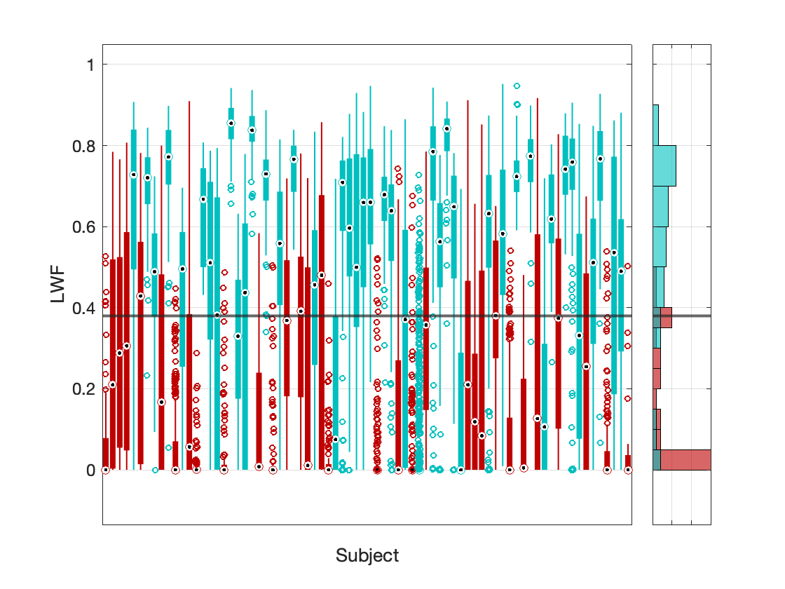
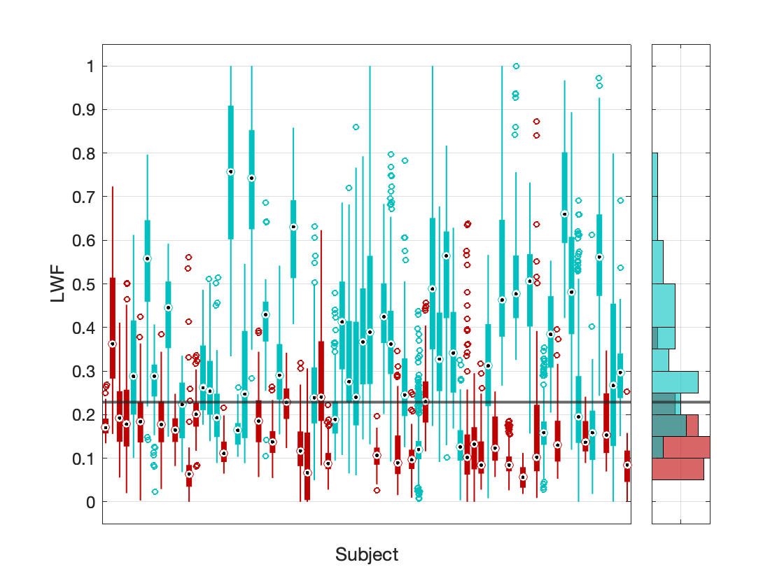
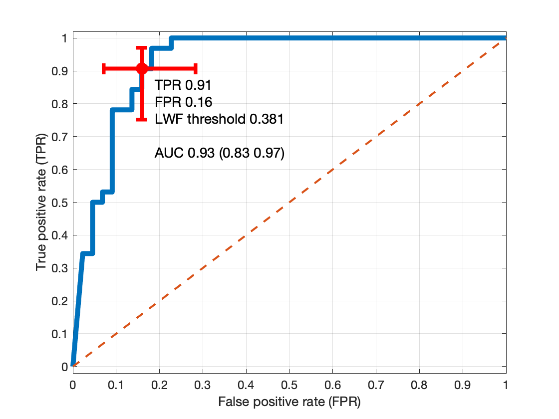
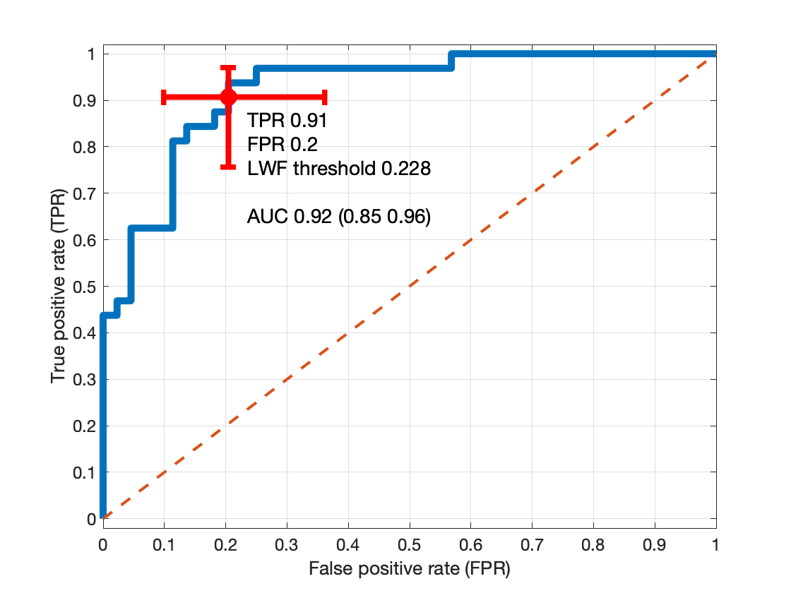
Box plots (25th-75th percentile) of the LWF within the lesion ROI for each subject were calculated from the first 8 echoes using the NNLS method and a histogram of median ROI values are shown in Figure 1. Data from the rapid fit is shown in Figure 2. The greater spread of values for the NNLS method is likely due to the ill-posed nature of the problem (many T2 distributions can give a similar prediction of the signal).ROC curves for the two fits are shown in Figs 3 and 4. The ROC AUCs are 0.93 and 0.92 suggesting that the fit performance of each fit is similar.
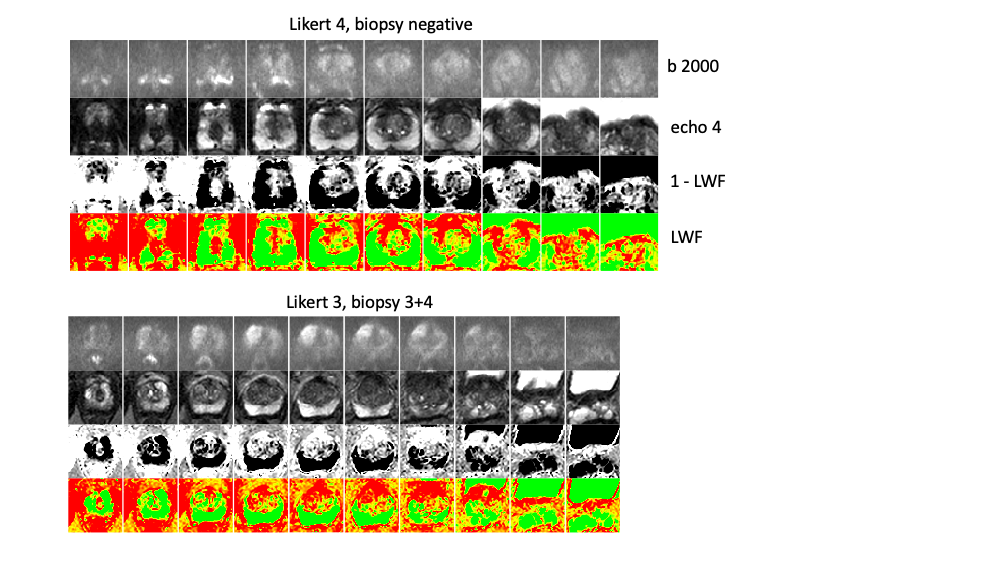
Figure 5 shows example data from the 8-echo, 17 slice data for two patients.
Discussion and Conclusion
Limitations: A single-centre, single-reader study with biopsy data only from men with a Likert score of 3 or higher. ROIs were identified using routine mpMRI scans and the study does not evaluate the use of LWF as an isolated test. The ROC AUCs are in-sample estimates and further test data is required to assess the method prospectively.Reasons for mis-classification were not formally analysed, but some ROIs were noted to include tissue with both high and low LWF (the LWF maps were not used during ROI placement) and the method appears to be better in focal peripheral zone lesions than larger regions located in the central and transition zones.
Our data from 76 patients suggests that a rapid LWF fitting achieves a near-instant fit with similar ability to discriminate clinically significant prostate cancer to a slower, commonly used alternative.
Acknowledgements
The INNOVATE study is supported by Prostate Cancer UK: Targeted Call 2014: Translational Research St.2, project reference PG14-018-TR2. Philips provided research support.References
Atkinson D, Gong Y, Brembilla G, Punwani S. Rapid fitting of Luminal Water Fraction in Prostate MRI. ISMRM 2021, p. 4088.
Bjarnason, T.A. and Mitchell, JR. (2010). AnalyzeNNLS: Magnetic resonance multiexponential decay image analysis. Journal of Magnetic Resonance, 206(2), 200-204. (https://sourceforge.net/projects/analyzennls/ Version MacVer-2.5.1)
Chan RW, Lau AZ, Detzler G, Thayalasuthan V, Nam RK, Haider MA. Evaluating the accuracy of multicomponent T2parameters for luminal water imaging of the prostate with acceleration using inner-volume 3D GRASE. Magn Res Med. 2019. 81(1) 466-476. DOI: 10.1002/mrm.27372.
Devine W, Giganti F, Johnston EW, Sidhu HS, Panagiotaki E, Punwani S, Alexander DC, Atkinson D. Simplified Luminal Water Imaging for the Detection of Prostate Cancer From Multiecho T2 MR Images. J Magn Reson Imaging. 2019: 50(3):910-917. DOI: 10.1002/jmri.26608
Hectors S, Said D, Gnerre J, Tewari A, Taouli B. Luminal Water Imaging: Comparison With Diffusion-Weighted Imaging (DWI) and PI-RADS for Characterization of Prostate Cancer Aggressiveness. J. Magn. Reson. Imaging 2020;52:271–279. DOI: 10.1002/jmri.27050
Johnston et al (2016). INNOVATE: A prospective cohort study combining serum and urinary biomarkers with novel diffusion-weighted magnetic resonance imaging for the prediction and characterisation of prostate cancer. BMC Cancer 16:816 DOI: 10.1186/s12885-016-2856-2
Sabouri, S., Fazli, L., Chang, S.D., Savdie, R., Jones, E.C., Goldenberg, S.L., Black, P.C. and Kozlowski, P. (2017). MR measurement of luminal water in prostate gland: Quantitative correlation between MRI and histology. Journal of Magnetic Resonance Imaging, 46(3), pp.861–869. DOI 10.1002/jmri.25624
Figures