0802
Estimating perfusion and permeability using neural network with training data generated from vessel construction and transport simulation1Cornell University, Ithaca, NY, NY, United States, 2Cornell University, New York, NY, United States, 3Weill Cornell Medical College, New York, NY, United States
Synopsis
We propose to estimate perfusion parameters (perfusion $$$F$$$, permeability $$$K^{trans}$$$, vascular space volume $$$V_p$$$ and extravascular extracellular volume $$$V_e$$$) from contrast enhanced MRI using Quantitative Transport and Exchange network (QTEnet), a deep learning method that does not require an arterial input function. Training data were generated by solving the transport equation in simulated high-resolution vasculature and computing the corresponding 4D tracer propagation. A 3D U-net was trained to reconstruct perfusion parameters from the tracer propagation images. Tracer propagation simulated in experimentally obtained tumor vasculature was used for valiation, and the method was then applied to glioma DCE MRI data.
Introduction
Quantitative transport mapping (QTM) method was proposed recently to overcome the dependence of kinetic modeling method on arterial input function (AIF)1,2,3. However, when applied to multi compartment kinetic modeling, the nonlinearity of the problem makes the inversion highly dependent on the initial guess. To overcome this problem, we propose to estimate perfusion parameters (perfusion $$$F$$$ permeability $$$K^{trans}$$$ , vascular space volume $$$V_p$$$ and extravascular extracellular space volume $$$V_e$$$ ) from contrast enhanced MR images using a deep neural network (quantitative transport and exchange network, QTEnet). To generate training data, a large set of simulated high resolution 3D vascular geometries containing arteries, capillaries and veins were generated based on constrained constructive optimization (CCO)4 and randomly generated perfusion parametric maps. Tracer propagation inside each of these vascular geometries and the surrounding extravascular space was simulated using transport equation with parabolic flow assumption ignoring diffusion. The performance of the network was tested on simulated concentration profile in an experimentally obtained tumor vascular geometry and in glioma DCE MRI images.Methods
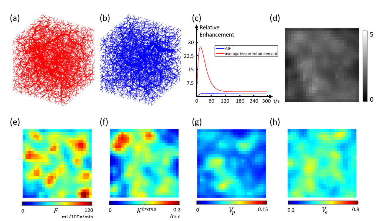
We considered the vasculature and tracer propagation inside a 32*32*32 mm3 volume. perfusion $$$F$$$ permeability $$$K^{trans}$$$ , vascular space volume $$$V_p$$$ and extravascular extracellular space volume $$$V_e$$$ were randomly generated using a mixed Gaussian spatial distribution: $$$F(\mathbf{x})=\sum_{i=1}^{N_0}e^{-\frac{(x-x_i)^2}{(R_i^2) }} $$$.Here $$$\mathbf{x}=[x,y,z] $$$ is the 3D coordinate, $$$N_0$$$ =100 the number of Gaussian kernels, $$$x_i$$$ the kernel locations and $$$R_i$$$ the kernel radii.$$$x_i$$$ and $$$R_i$$$ were chosen from a uniform distribution between 0mm to 3.2mm and 1mm to 3mm, respectively. $$$K^{trans}$$$ ,$$$V_p$$$ and $$$V_e$$$ were simulated in the same way. Afterwards, $$$F$$$ , $$$K^{trans}$$$ ,$$$V_p$$$ and $$$V_e$$$ were scaled to 0-150 mL/100g/min, 0-0.25/min, 0.01-0.1 and 0.3-0.7 respectively based on the range of these parameters measured in tumor5-8. Examples of the generated perfusion parameter maps are shown in Figures 1c-f. After the parametric maps were determined, the arteries, capillaries and veins were built using constrained constructive optimization (CCO) method4. Example arterial and venous vascular geometries are shown in Figures 1a-b. After the flow for each vessel segment was determined, tracer propagation in the vascular network was simulated using transport equation assuming no diffusion, parabolic flow in arteries and veins, plug flow in capillaries, and a constant exchange rate ( $$$K^{trans}$$$ ) between capillary and extravascular space9. A concentration $$$c(t)=k_1te^{(-t/k_2)}+k_3(1-e^{-t/k_4}) $$$ was used as the arterial supply for the purposes of simulation. For each training data, $$$k_1$$$,$$$k_3$$$ were chosen from a random distribution from 2 to 6, $$$k_2$$$,$$$k_4$$$ were chosen from a random distribution from 10 to 20, which represents maximum enhancement from 4 to 12 and mean transit time from 10s to 40s. An example arterial supply and corresponding simulated concentration at 40s are shown in Figures 1c and 1d, respectively.
A 28-layer 3D U-net was chosen as network architecture10. Concentration data at different time point were concatenated as features in the input. The loss function was set as L1 norm of network output and ground truth of the parameters. The network weights were optimized using Adam method with epoch=40, batch number=1, learning rate=0.001.
Concentration data simulated in artificial vessel networks (test data) and in tumor vessel network (obtained from optical projection tomography image of mice colorectal carcinoma) were used to test the performance of the network11. DCE MRI images in 10 patients with high grade glioma were acquired using a T1 fast-low angle shot, FLASH/vibe sequence. The scanning parameters were as follows: 40 dynamic acquisitions, 4.9 s per dynamic acquisition, TR=4.09 ms, TE=1.47 ms, flip angle=9°, phase=75%, bandwidth=400 Hz, thickness=4 mm, slice gap=0 mm, FOV=180*180 mm2, matrix=192×144, TA=245s. As the input size of the neural network is 32×32×32, the DCE MRI images were interpolated to 1mm voxel size. The network was repeatedly applied in a sliding window fashion (step size =4 voxels) across the entire volume. As a comparison, two compartment kinetic modeling method was also used to calculate $$$F$$$ , $$$K^{trans}$$$ ,$$$V_p$$$ and $$$V_e$$$ 9.
Results
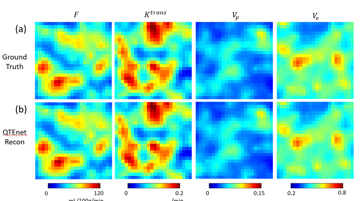
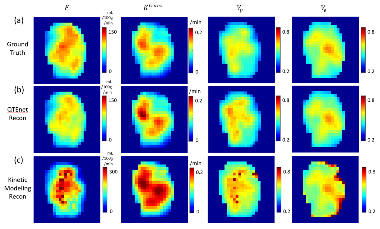
Our proposed QTEnet method can accurately reconstruct and from simulated 4D concentration profile using artificial and tumor vasculature. QTEnet reconstruction results in artificial vasculature is shown in Figure 2b. The relative root mean squared error (rRMSE) of $$$F$$$ is 3.00%, $$$K^{trans}$$$ is 3.87%, $$$V_p$$$ is 3.64%, and $$$V_e$$$ is 5.62%.The QTEnet results for simulated tracer data in the experimentally obtained tumor vasculature is shown in Figure 3, and QTEnet reconstruction results from tumor vasculature are shown in figure 4b. The rRMSE of is $$$F$$$ 12.87%, $$$K^{trans}$$$ is 6.92%, $$$V_p$$$ is 9.28%, and $$$V_e$$$ is 4.01%. As a comparison, parameter reconstruction using kinetic modeling are shown in Figure 4c. The corresponding rRMSE of $$$F$$$ is 56.22%, $$$K^{trans}$$$ is 13.63%, $$$V_p$$$ is 26.14%, and $$$V_e$$$ is 36.74%.
QTEnet and kinetic modeling applied to DCE MRI images of a high-grade glioma are shown in Figure 5. QTEnet appears less noisy compared kinetic modeling. Tumor showed a higher and compared to normal tissue.
Discussion and Conclusion
We present here a perfusion parameter estimation method based on deep learning using simulated vasculature and tracer propagation as training data. The proposed QTEnet method can accurately reconstruct $$$F$$$ , $$$K^{trans}$$$, $$$V_p$$$and $$$V_e$$$ for different vasculature in simulated data. When applied to DCE MRI, QTEnet can reconstruct these perfusion parameters with good image quality fully automatically.Acknowledgements
The author has no acknowledgements.References
(1) Zhou, Liangdong, Qihao Zhang, Pascal Spincemaille, Thanh D. Nguyen, John Morgan, Weiying Dai, Yi Li, Ajay Gupta, Martin R. Prince, and Yi Wang. "Quantitative transport mapping (QTM) of the kidney with an approximate microvascular network." Magnetic resonance in medicine 85, no. 4 (2021): 2247-2262.
(2) Zhang, Qihao, Pascal Spincemaille, Michele Drotman, Christine Chen, Sarah Eskreis-Winkler, Weiyuan Huang, Liangdong Zhou et al. "Quantitative transport mapping (QTM) for differentiating benign and malignant breast lesion: Comparison with traditional kinetics modeling and semi-quantitative enhancement curve characteristics." Magnetic Resonance Imaging (2021).
(3) Kety SS. The theory and application of the exchange of inert gas at the lungs and tissues. Pharmacol rev 1951;3:1-41
(4) Karch R, Neumann F, Neumann M, Schreiner W. A three-dimensional model for arterial tree representation, generated by constrained constructive optimization. Computers in biology and medicine 1999;29(1):19-38.
(5) Law M, Yang S, Babb JS, Knopp EA, Golfinos JG, Zagzag D, Johnson G. Comparison of cerebral blood volume and vascular permeability from dynamic susceptibility contrast-enhanced perfusion MR imaging with glioma grade. American Journal of Neuroradiology 2004;25(5):746-755
(6) Yoo RE, Choi SH, Cho HR, Kim TM, Lee SH, Park CK, Park SH, Kim IH, Yun TJ, Kim JH. Tumor blood flow from arterial spin labeling perfusion MRI: A key parameter in distinguishing high‐grade gliomas from primary cerebral lymphomas, and in predicting genetic biomarkers in high‐grade gliomas. Journal of Magnetic Resonance Imaging 2013;38(4):852-860.
(7) Reynaud O, Winters KV, Hoang DM, Wadghiri YZ, Novikov DS, Kim SG. Pulsed and oscillating gradient MRI for assessment of cell size and extracellular space (POMACE) in mouse gliomas. NMR in biomedicine 2016;29(10):1350-1363. (8) Zhou, Liangdong, Qihao Zhang, Pascal Spincemaille, Thanh D. Nguyen, John Morgan, Weiying Dai, Yi Li, Ajay Gupta, Martin R. Prince, and Yi Wang. "Quantitative transport mapping (QTM) of the kidney with an approximate microvascular network." Magnetic resonance in medicine 85, no. 4 (2021): 2247-2262.
(8) Aronen HJ, Gazit IE, Louis DN, Buchbinder BR, Pardo FS, Weisskoff RM, Harsh GR, Cosgrove G, Halpern EF, Hochberg FH. Cerebral blood volume maps of gliomas: comparison with tumor grade and histologic findings. Radiology 1994;191(1):41-51.
(9) Sourbron SP, Buckley DL. On the scope and interpretation of the Tofts models for DCE‐MRI. Magnetic resonance in medicine 2011;66(3):735-745.
(10) Ronneberger O, Fischer P, Brox T. U-net: Convolutional networks for biomedical image segmentation. 2015. Springer. p 234-241.
(11) d’Esposito A, Sweeney PW, Ali M, Saleh M, Ramasawmy R, Roberts TA, Agliardi G, Desjardins A, Lythgoe MF, Pedley RB. Computational fluid dynamics with imaging of cleared tissue and of in vivo perfusion predicts drug uptake and treatment responses in tumours. Nature Biomedical Engineering 2018;2(10):773-787.
Figures