0789
Comparing the SPIJN algorithm for myelin water fraction mapping with conventional NNLS evaluation in healthy and multiple sclerosis brains
Ronja C. Berg1, Thomas Amthor2, Irene Vavasour3, Mariya Doneva2, and Christine Preibisch1
1Department of Neuroradiology, School of Medicine, Technical University of Munich, Munich, Germany, 2Philips Research Europe, Hamburg, Germany, 3Department of Radiology, University of British Columbia, Vancouver, BC, Canada
1Department of Neuroradiology, School of Medicine, Technical University of Munich, Munich, Germany, 2Philips Research Europe, Hamburg, Germany, 3Department of Radiology, University of British Columbia, Vancouver, BC, Canada
Synopsis
Myelin water fraction (MWF) mapping provides information on myelin concentration, which can be affected by neurological diseases. Most commonly, a non-negative least squares (NNLS) algorithm is used to obtain MWF. A faster alternative is the Sparsity Promoting Iterative Joint NNLS (SPIJN) algorithm. Here, we compared both methods in several brain regions from healthy participants and normal-appearing and lesion tissue from MS patients (EDSS 0-1.5). We found that NNLS-based lesion-average MWF was rather comparable to white matter while SPIJN-based MWF was lower. Thus, SPIJN could be more sensitive to demyelination in lesions but comparisons to gold standard techniques are clearly needed.
Introduction
Various neurological diseases can affect and degrade myelin and thereby impair the conduction of nerve signals. One such disease is multiple sclerosis (MS), an inflammatory demyelinating disease that damages myelin and nerve fibers1. Precise knowledge of the myelin concentration is essential to better understand and treat such diseases. A valuable MRI based method for determining the myelin concentration is myelin water fraction (MWF) mapping2-3. Commonly, a non-negative least squares (NNLS) algorithm4 is used to calculate MWF from multi-echo spin-echo data. A new and faster method for MWF determination is the Sparsity Promoting Iterative Joint NNLS (SPIJN) algorithm5 that uses a joint sparsity constraint and enables inclusion of phase data. In a previous study, we investigated how the SPIJN algorithm (using either magnitude data only or complex data) compares to the NNLS method for MWF mapping in healthy WM regions6. Here, we additionally evaluated all three algorithms in a cohort of MS patients and investigated their performance in healthy, normal-appearing, and lesion tissue.Methods
Five healthy volunteers (aged 32±3y, 3f/2m) and five MS patients (aged 33±6y, 2f/3m; 4 relapsing-remitting MS, 1 clinically isolated syndrome; disease duration: 3-15y, average=9.4y; expanded disability status scale: 0-1.5, average =1.1) were scanned on a Philips 3T Ingenia Elition using a 32-channel head coil. The scan protocol comprised a 3D gradient- and spin-echo (GRASE) sequence for myelin water imaging (MWI), FLAIR, and MPRAGE. The scan parameters of the GRASE sequence were TE1/ΔTE/TR = 8/8/1120ms, 48 echoes, 1x2x5mm³ resolution, 20 slices, and a=90°. Data processing was performed using a non-negative least squares (NNLS) algorithm4 including stimulated echo correction7 and two variants of the Sparsity Promoting Iterative Joint NNLS5 algorithm. The mSPIJN variant used only magnitude data for MWF calculation, the cSPIJN variant additionally included phase information.In MS patients, lesions were segmented automatically using the lesion growth algorithm8 from the lesion segmentation tool9 for SPM1210. Lesions were defined as regions with lesion probabilities >0.5 and the peri-lesional tissue (‘Peri-Lesion’) as a 3-voxel wide shell surrounding lesions within normal-appearing white matter (WM). Whole-brain gray matter (GM) and WM masks were derived from MPRAGE data using SPM12’s segment module thresholded at tissue probability >0.5. Additionally, several WM tracts from the JHU DTI-based white-matter atlas11-12 were combined into five MW regions (corpus callosum, internal capsule, corona radiata, external capsule, and cingulum). All volumes-of-interest (VOIs) were co-registered to the GRASE data using either SPM12’s co-register (whole-brain GM and WM, lesion masks) or normalize module (JHU VOIs) and nearest-neighbor interpolation. Lesion-voxels were excluded from all non-lesion VOIs.
Results
MWF maps calculated using the three algorithms appeared visually similar. However, they slightly differed, especially in voxels segmented as lesions (Fig.1). In most lesions, SPIJN-based MWF was lower than NNLS-based MWF (Fig.2A-B). Phase like patterns can be seen in the difference and overlay images of cSPJIN and both NNLS and mSPJIN (Fig.2B-C). In most investigated VOIs, VOI-average MWF values from different MWF algorithms showed the same tendencies (highest MWF in the internal capsule and lowest in the external capsule and cingulum) across WM regions (Fig.3). However, MWF values of lesion segmentations were clearly decreased compared to WM MWF in both SPIJN variants, while NNLS-based MWF was rather comparable between lesions and WM (Fig.3). In non-lesion tissue, VOI-average MWF values were slightly higher for SPIJN reconstructions, especially for mSPIJN (Fig.3) and the pooled standard deviation across all voxels of all participants was slightly lower for SPIJN than for NNLS (Fig.4). Bland-Altman evaluations revealed highest agreement between both SPIJN algorithms and lowest agreement between NNLS and mSPIJN (Fig.5).Discussion
In healthy and normal-appearing brain regions, VOI-average SPIJN-based MWF was slightly higher than NNLS-based MWF. cSPIJN showed a somewhat better agreement with NNLS than mSPIJN probably achieved by eliminating bias when including phase data in the processing. Whole-brain WM and GM MWF values of all three methods correlated well with literature ranging from 0.118-0.156 in WM13-14 and 0.038±0.064 in GM13. Differences were found in the MWF of lesion segmentations with NNLS resulting in MWF values almost comparable to WM while SPIJN revealed much lower MWF values almost comparable to GM. Previous studies have found decreased average MWF in lesions compared to WM ranging mostly from 0.041 to 0.04613-15 but also reaching values up to 0.08516, which roughly correlate with our average lesion MWF. However, large differences have been reported between MWF values of individual lesions ranging between 0 and ~0.1114 or 0 and 0.1715. In this preliminary study including only five MS patients, it is hardly possible to determine why NNLS-based MWF yielded higher MWF in lesions than SPIJN-based MWF. One possible explanation could be a low degree of demyelination within the lesions of our cohort of MS patients that had a comparatively low EDSS (0-1.5). Further studies are urgently needed that compare not only NNLS3,17 but also SPIJN MWF in lesions with gold standard histology to evaluate the fidelity of MWF values from both methods.Conclusion
SPIJN yielded higher contrast between normal-appearing or healthy brain tissue and lesions compared to NNLS. Comparisons with gold standard techniques are needed to disentangle processing-based differences in MWF from microstructural effects influencing the degree of demyelination within lesions.Acknowledgements
Ronja Berg was supported by a PhD grant from the Friedrich-Ebert-Stiftung.References
- Bando, Y. (2020). Mechanism of demyelination and remyelination in multiple sclerosis. Clinical and Experimental Neuroimmunology, 11, 14-21.
- MacKay, A. L., & Laule, C. (2016). Magnetic resonance of myelin water: an in vivo marker for myelin. Brain plasticity, 2(1), 71-91.
- Laule, C., Leung, E., Li, D. K., Traboulsee, A. L., Paty, D. W., MacKay, A. L., & Moore, G. R. (2006). Myelin water imaging in multiple sclerosis: quantitative correlations with histopathology. Multiple Sclerosis Journal, 12(6), 747-753.
- MacKay, A., Laule, C., Vavasour, I., Bjarnason, T., Kolind, S., & Mädler, B. (2006). Insights into brain microstructure from the T2 distribution. Magnetic resonance imaging, 24(4), 515-525.
- Nagtegaal, M., Koken, P., Amthor, T., de Bresser, J., Mädler, B., Vos, F., & Doneva, M. (2020). Myelin water imaging from multi-echo T2 MR relaxometry data using a joint sparsity constraint. NeuroImage, 219, 117014.
- Berg, R., Amthor, T., Vavasour, I., Donea, M., & Preibisch, C. (2020). Comparing the SPIJN algorithm with conventional NNLS for myelin water fraction mapping. ESMRMB Abstract #1118.
- Prasloski, T., Mädler, B., Xiang, Q. S., MacKay, A., & Jones, C. (2012). Applications of stimulated echo correction to multicomponent T2 analysis. Magnetic resonance in medicine, 67(6), 1803-1814.
- Schmidt, P., Gaser, C., Arsic, M., Buck, D., Förschler, A., Berthele, A., ... & Mühlau, M. (2012). An automated tool for detection of FLAIR-hyperintense white-matter lesions in multiple sclerosis. Neuroimage, 59(4), 3774-3783.
- Lesion Segmentation Tool for SPM https://www.applied-statistics.de/lst.html
- Statistical Parametric Mapping: http://www.fil.ion.ucl.ac.uk/spm
- JHU DTI-based white-matter atlases https://identifiers.org/neurovault.collection:264
- Mori, S., Wakana, S., Van Zijl, P. C., & Nagae-Poetscher, L. M. (2005). MRI atlas of human white matter. Elsevier, Amsterdam, The Netherlands (2005).
- Mackay, A., Whittall, K., Adler, J., Li, D., Paty, D., & Graeb, D. (1994). In vivo visualization of myelin water in brain by magnetic resonance. Magnetic resonance in medicine, 31(6), 673-677.
- Vavasour, I. M., Whittall, K. P., Mackay, A. L., Li, D. K., Vorobeychik, G., & Paty, D. W. (1998). A comparison between magnetization transfer ratios and myelin water percentages in normals and multiple sclerosis patients. Magnetic resonance in medicine, 40(5), 763-768.
- Laule, C., Vavasour, I. M., Moore, G. R. W., Oger, J., Li, D. K., Paty, D. W., & MacKay, A. L. (2004). Water content and myelin water fraction in multiple sclerosis. Journal of neurology, 251(3), 284-293.
- Oh, J., Han, E. T., Lee, M. C., Nelson, S. J., & Pelletier, D. (2007). Multislice brain myelin water fractions at 3T in multiple sclerosis. Journal of Neuroimaging, 17(2), 156-163.
- Moore, G. R. W., Leung, E., MacKay, A. L.,
Vavasour, I. M., Whittall, K. P., Cover, K. S., ... & Paty, D. W. (2000). A
pathology-MRI study of the short-T2 component in formalin-fixed multiple
sclerosis brain. Neurology,
55(10), 1506-1510.
Figures
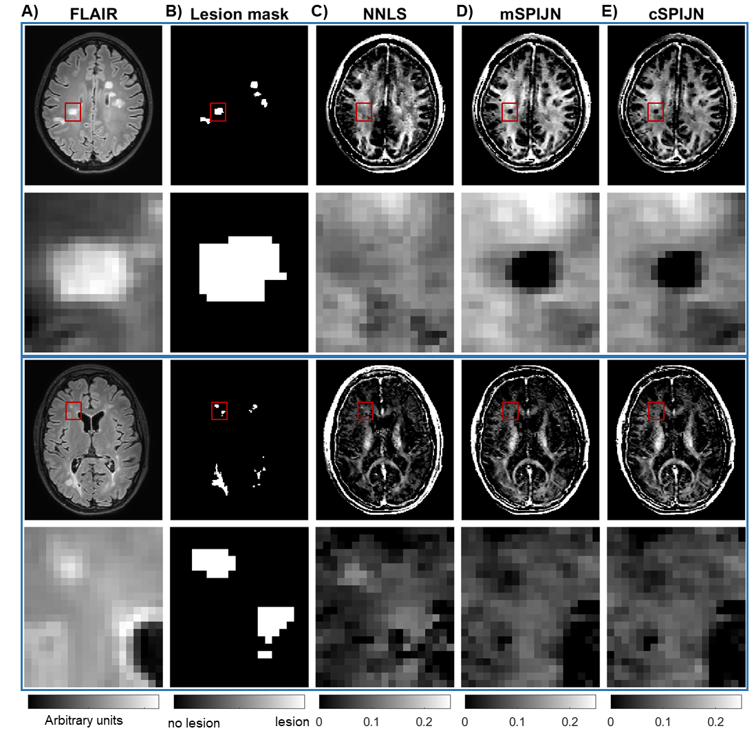
Figure
1: Exemplary slices of FLAIR images (A), lesion segmentations (B), and myelin
water fraction (MWF) maps of two different MS patients including zoomed-in
regions of lesion segmentations. MWF maps are shown for NNLS evaluations (C),
magnitude-based SPIJN (D), and complex-data-based SPIJN (E). Red rectangles in
the first and third rows indicate the location of the zoomed-in regions in the
second and last rows.
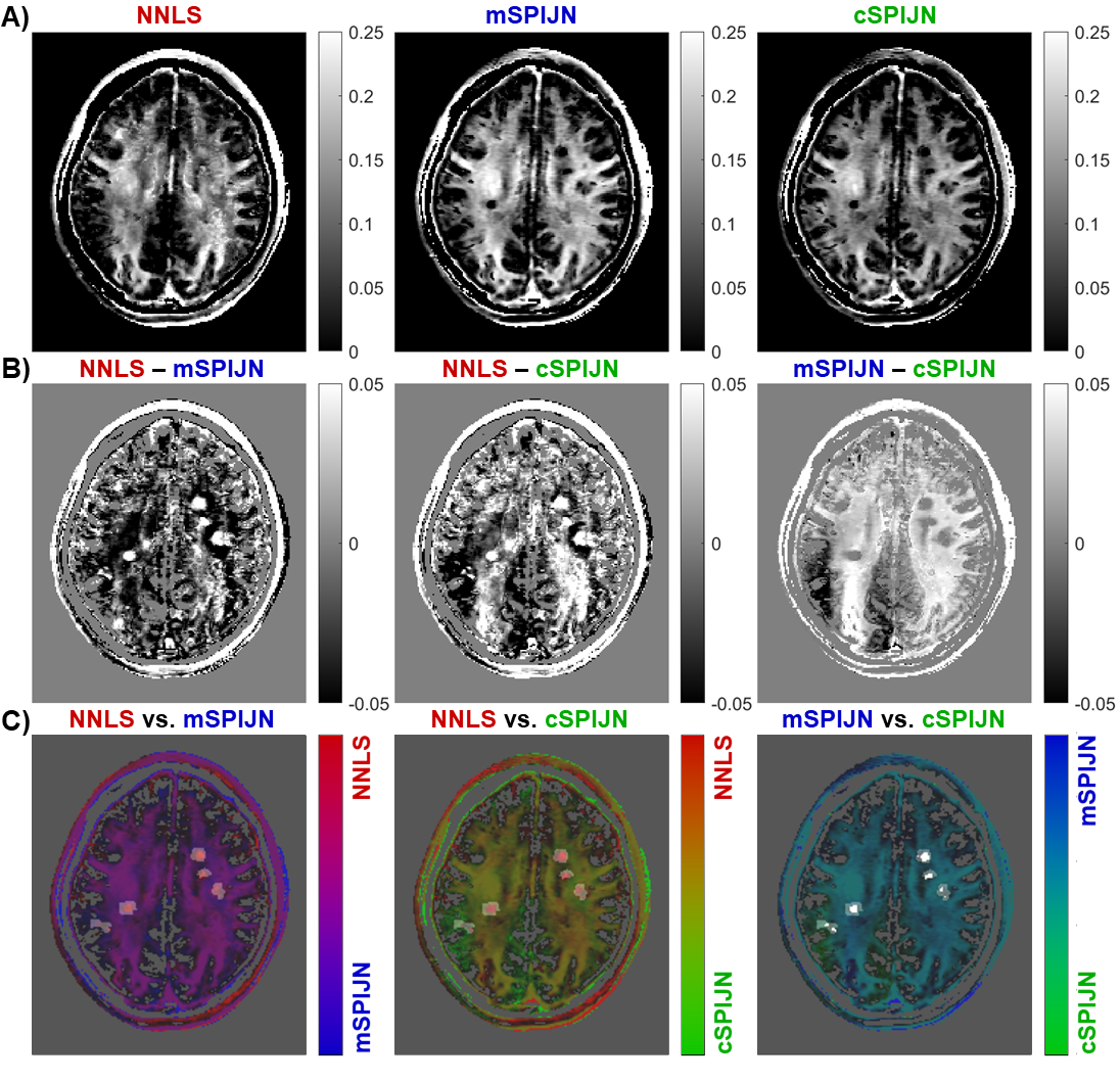
Figure
2: Visual comparison of MWF maps calculated by the NNLS algorithm and both variants of the SPIJN algorithm
(A), difference images (B), and overlays (C) using pairs of MWF maps shown in (A). The
same slice is shown as in the first row of Figure 1. Differences in (B) are
shown as absolute differences (in units of the MWF) with dark black areas representing negative difference and bright white areas positive difference. In
(C), pairs of MWF maps are overlaid on the lesion mask.
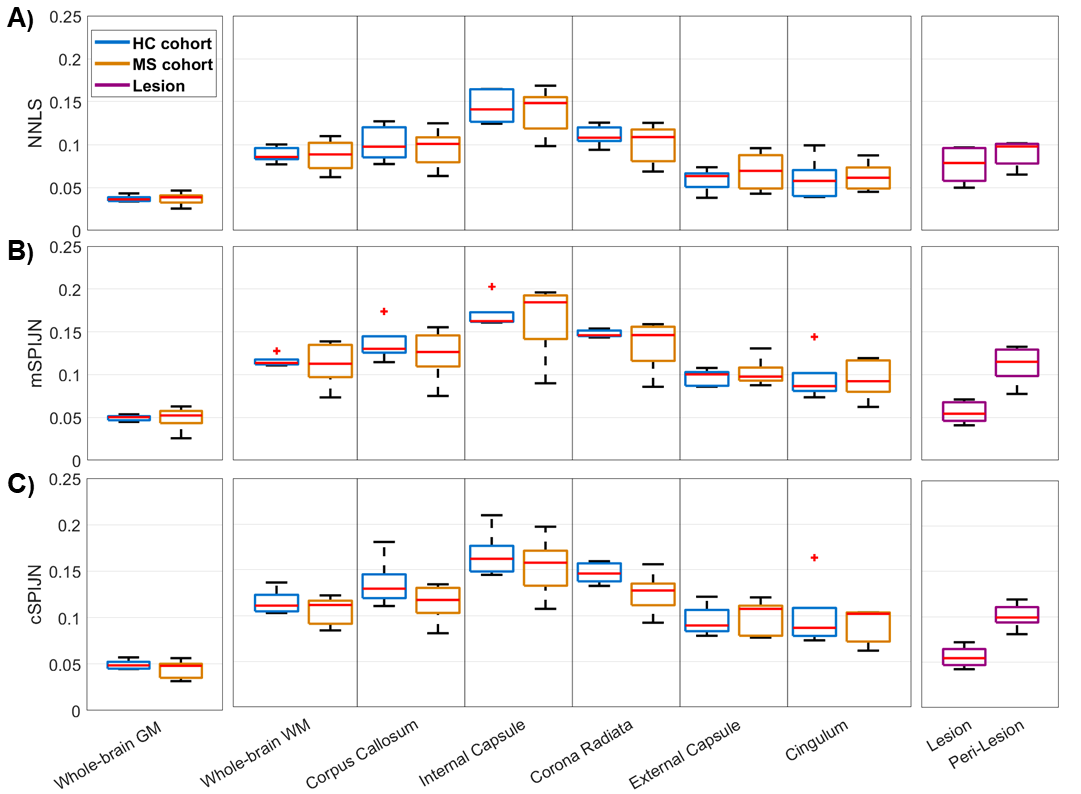
Figure
3: Boxplots of VOI-average MWF values calculated using NNLS (A), mSPIJN (B), or
cSPIJN (C) from different tissue types or brain
regions. Each boxplot contains five VOI-average values
either from five healthy volunteers (blue) or from five MS patients in
normal-appearing tissue (orange), in lesions (purple), or in peri-lesional
normal-appearing white matter (purple). Red lines indicate the median of mean
values, boxes (25th and 75th percentiles) and whiskers indicate standard
deviation across participants.
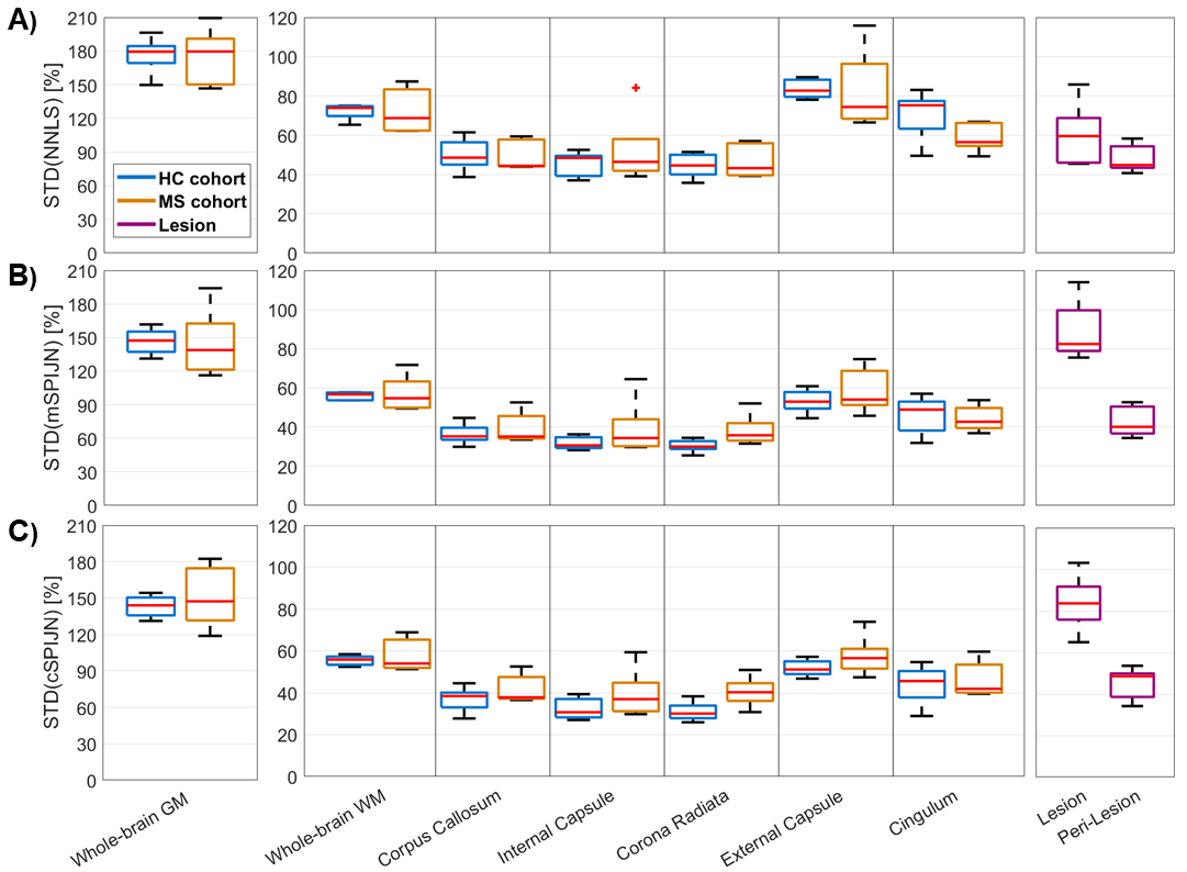
Figure
4: Boxplots showing standard deviations of MWF values calculated using NNLS
(A), mSPIJN (B), or cSPIJN (C) and evaluated within different tissue types or
brain regions. Each boxplot contains five VOI-mean standard
deviation values either from five healthy volunteers (blue) or from five MS
patients in normal-appearing tissue (orange), in lesions (purple), or in peri-lesional
normal-appearing white matter (purple). Red lines indicate the median of mean
values, boxes (25th and 75th percentiles) and whiskers indicate standard
deviation across participants.
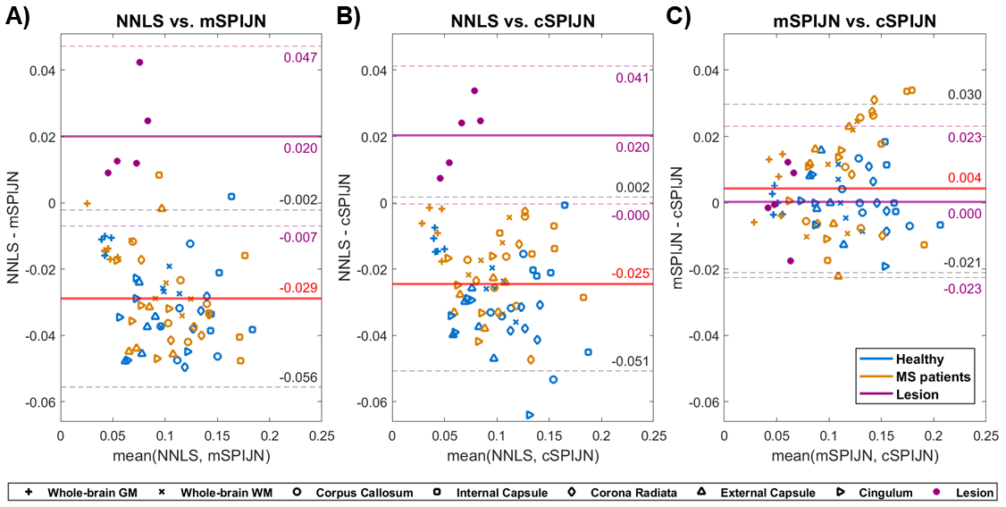
Figure
5: Bland-Altman plots comparing VOI-average MWF values between pairs of MWF
algorithms including NNLS vs. mSPIJN (A), NNLS vs. cSPIJN (B), and mSPIJN vs.
cSPIJN (C). Each panel contains two Bland-Altman plots showing
VOI-mean MWF values from healthy participants and MS patients. The Bland-Altman
evaluation based on both healthy (blue) and normal-appearing (orange) tissue is
shown with red and black lines; the one based on lesion data with purple lines.
Average difference values (solid lines) and 95% limits of agreement (± 1.96
standard deviation, dashed lines) are provided.
DOI: https://doi.org/10.58530/2022/0789