0765

Axonal diffusivities from two-shell PGSE data

Marco Pizzolato^1,2,3, Mariam Andersson³, Erick Jorge Canales-Rodríguez², and Tim Bjørn Dyrby^1,3
¹Department of Applied Mathematics and Computer Science, Technical University of Denmark, Kgs. Lyngby, Denmark, ²Signal Processing Lab (LTS5), École Polytechnique Fédérale de Lausanne, Lausanne, Switzerland, ³Danish Research Centre for Magnetic Resonance, Copenhagen University Hospital - Amager and Hvidovre, Copenhagen, Denmark

Synopsis

The strongly diffusion-weighted MRI signal contains information about the axonal parallel and perpendicular diffusivities. Powder averaging has simplified the estimation of the perpendicular diffusivity, however it is difficult to estimate the parallel one because, as we show, the powder-averaged signal at strong diffusion weightings is insensitive to it. In this work we propose a method that enables the estimation of both diffusivities from only two conventional linear PGSE signal shells collected at high b-values. The method is tested on public MGH-HCP data to retrieve axonal diffusivities and calculate the MR radius in white matter.

INTRODUCTION

The use of high diffusion-weighting regimes, i.e. high b-values, coupled with powder averaging of the signal acquired along uniformly distributed directions, has largely simplified the task of estimating the perpendicular diffusivity of axons in white matter¹. While high b-values entail that the diffusion-weighted magnetic resonance signal in a white matter voxel arises primarily from the axonal compartment (excluding myelin due to the use of high echo times)², powder averaging removes the need to model orientational dispersion effects and the presence of multiple fiber bundles³. When representing the signal decay of the axonal compartment with an axisymmetric diffusion tensor, defined by parallel and perpendicular diffusivities ($$$\lambda_{\parallel}$$$,$$$\lambda_{\perp}$$$), the use of high b-values enables us to approximate the powder-averaged axonal signal with a modified power law¹ which conveniently removes the need for estimating the parallel diffusivity, thus enabling a straightforward estimation of the perpendicular one. This advantage, however, also constitutes the fundamental reason why the high b-value powdered-averaged signal is inherently insensitive to the parallel diffusivity⁴, which cannot be reliably estimated. Alternative methods⁵ employ "prolate" tensor encoding (e.g. trough triple diffusion encoding) in addition to "linear" conventional Pulsed Gradient Spin Echo⁶ (PGSE) data to recover the parallel diffusivity while assuming, however, a negligible perpendicular diffusivity ($$$\lambda_{\perp}=0$$$).

We present a method for estimating both parallel and perpendicular diffusivities based on only two PGSE (linear) shells. Linear data has higher efficiency in diffusion gradient usage allowing to minimize the echo time, thus increasing the effective signal-to-noise ratio (SNR), and has optimal directional resolution⁷.

METHODS

The representation of the axonal signal at b-value $$$b$$$ along a direction $$$\vec{u}$$$ is⁸
$$S_a(b,\vec{u}) = C \sum_{l=0,even}^{L} \sum_{m=-l}^{l} c^{'}_{lm} 2\pi e^{-b\lambda_{\perp}} \Psi_l\left(b[\lambda_{\parallel}-\lambda_{\perp}]\right) Y_l^m(\vec{u})$$
where $$$C$$$ is a constant that includes proton density, relaxation effects, and the axonal volume fraction, $$$c^{'}_{lm}$$$ are the spherical harmonics coefficients of the orientation distribution function expanded up to zonal order $$$L$$$, $$$Y_l^m$$$ is the real spherical harmonic basis⁹ of order $$$l$$$ and $$$m$$$, and where $$$\Psi_l$$$ are the solutions of $$$\int_{-1}^{1}P_l(\xi)e^{-\xi t^2}dt$$$ with $$$P_l$$$ being the $$$l$$$-order Legendre polynomial.
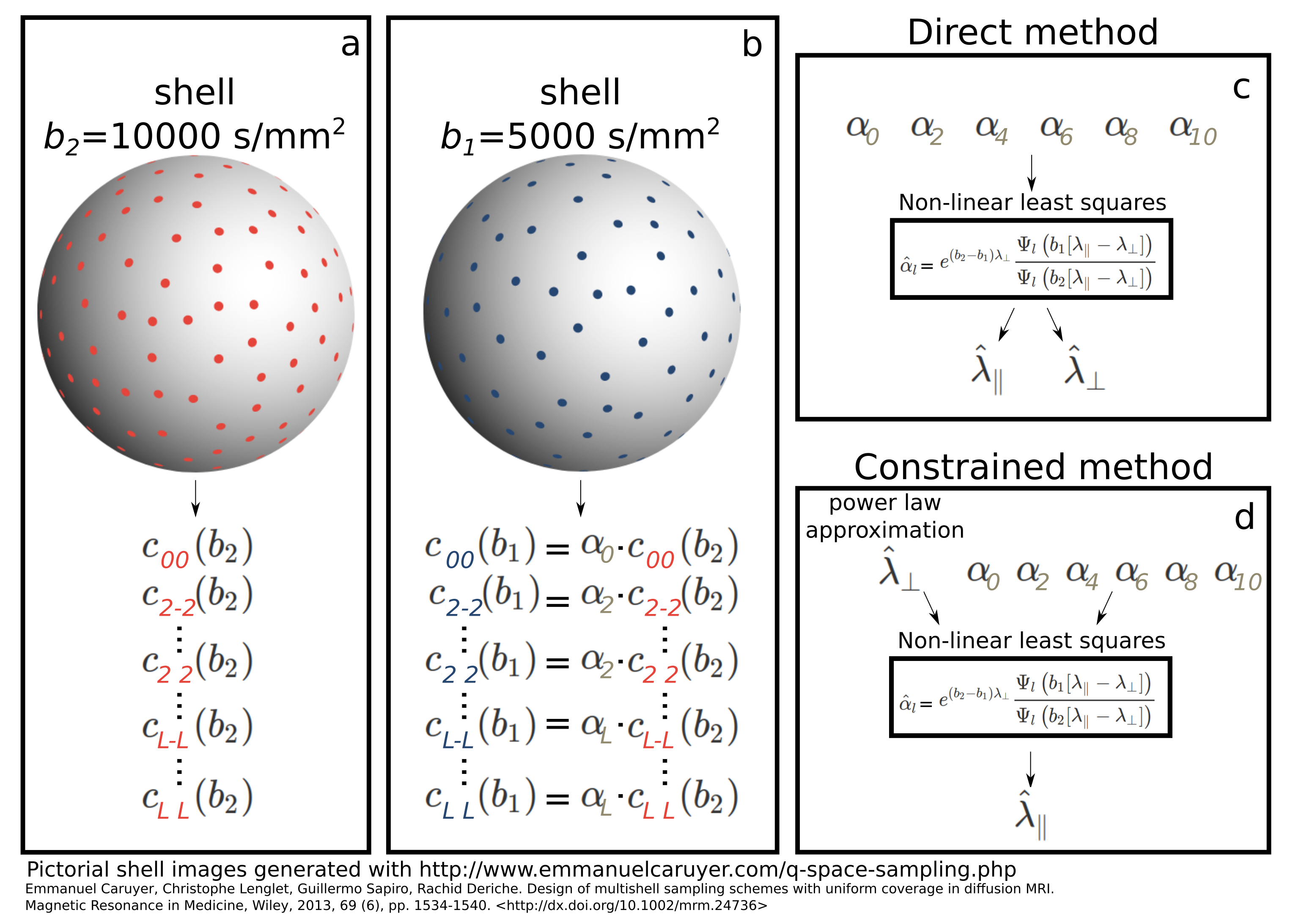
The proposed method considers the expansion in spherical harmonics of two PGSE shells acquired at high b-value, $$$b_2>b_1>>0$$$. We first expand the signal at $$$b_2$$$
$$S(b_2,\vec{n}) = \sum_{l=0,even}^{L} \sum_{m=-l}^{l} c_{lm}(b_2) Y_{l}^{m}(\vec{n})$$
recognizing that
$$c_{lm}(b_2) = c^{'}_{lm} C 2\pi e^{-b_2\lambda_{\perp}} \Psi_l\left(b_2[\lambda_{\parallel}-\lambda_{\perp}]\right)$$
and analogously
$$c_{lm}(b_1) = c^{'}_{lm} C 2\pi e^{-b_1\lambda_{\perp}} \Psi_l\left(b_1[\lambda_{\parallel}-\lambda_{\perp}]\right)$$
from which we observe that the ratio
$$\alpha_l(b_1,b_2,\lambda_{\parallel},\lambda_{\perp}) := \frac{c_{lm}(b_1)}{c_{lm}(b_2)} = e^{(b_2-b_1) \lambda_{\perp}} \frac{ \Psi_l\left(b_1[\lambda_{\parallel}-\lambda_{\perp}]\right)}{ \Psi_l\left(b_2[\lambda_{\parallel}-\lambda_{\perp}]\right)} $$
only depends on $$$\lambda_{\parallel}$$$ and $$$\lambda_{\perp}$$$ since the parts that do not depend on b-value (relaxation, proton density, volume fraction) are factored out. We then expand the signal at $$$b_1$$$ using the ratio $$$\alpha_l$$$
$$S(b_1,\vec{n}) = \sum_{l=0,even}^{L} \sum_{m=-l}^{l} \alpha_l(b_1,b_2,\lambda_{\parallel},\lambda_{\perp}) c_{lm}(b_2) Y_{l}^{m}(\vec{n}).$$
By obtaining the estimates $$$\hat{c}_{lm} (b_2)$$$ via linear least squares, eventually regularized⁹, we create the design matrix $$$A$$$ for the latter problem with entries $$$A_{ij}=\hat{c}_{j}(b_2)Y_{j}(\vec{n}_i)$$$ where $$$i$$$ iterates over the $$$N\ge(L+2)/2$$$ directions for the shell at $$$b_1$$$ and $$$j$$$ over all allowed combinations of indices $$$l$$$ and $$$m$$$. We then solve the linear problem $$$\textbf{s}=\textbf{A}\textbf{a}$$$ for the vector of coefficients $$$\textbf{a}=[\alpha_0,\alpha_2,...,\alpha_L]^T$$$ having $$$\textbf{s}=[S(b_1,\vec{n}_1),S(b_1,\vec{n}_2),...,S(b_1,\vec{n}_N))]^T$$$. Using non-linear least squares we finally obtain the estimates $$$\hat{\lambda}_\parallel$$$ and $$$\hat{\lambda}_\perp$$$ from the estimated ratios $$$\hat{\alpha}_l$$$ using the corresponding analytic expression indicated earlier. We evince that $$$L\ge2$$$ is required. Two different estimation procedures, the direct and constrained methods, are illustrated in Fig. 1 and described in the caption.

RESULTS

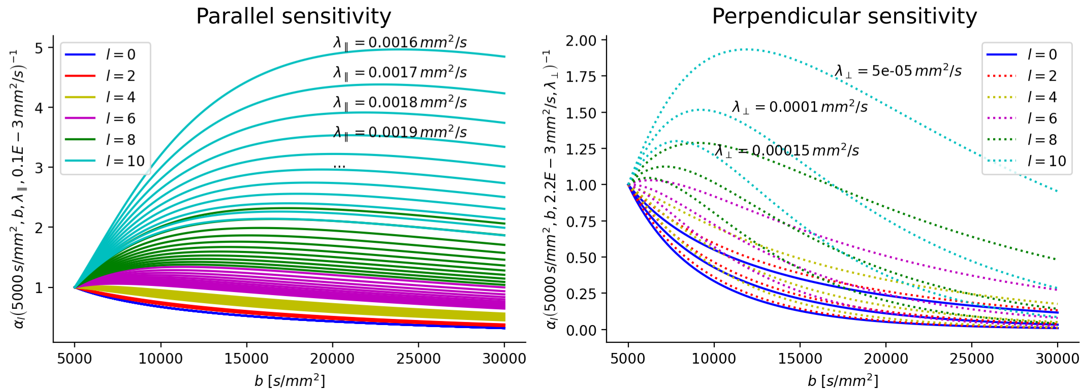
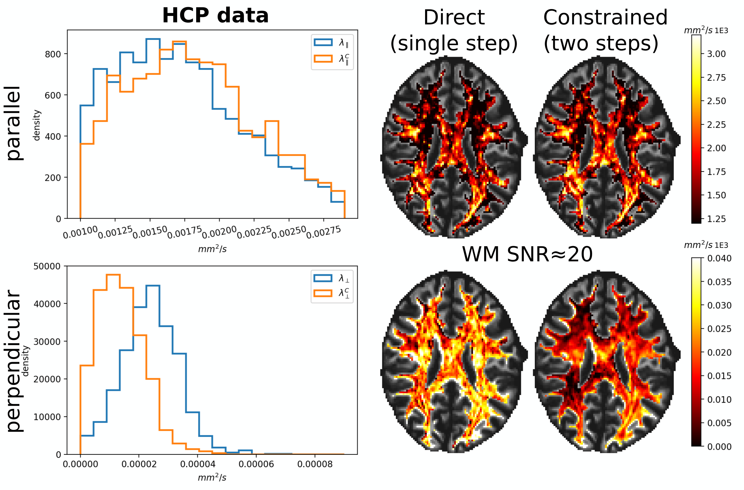
Fig. 2 illustrates the sensitivity of the ratio $$$\alpha_l$$$ as a function of $$$\lambda_{\parallel}$$$ and $$$\lambda_{\perp}$$$ for different values of $$$l$$$ and calculated for $$$b_1=5000\,\textrm{s/mm}^2$$$ and for $$$b_2\in]5000,10000]\,\textrm{s/mm}^2$$$. The extrema of the range were fixed according to the acquisition protocol for the MGH adult diffusion data of the Human Connectome Project (MGH-HCP), which we used for the in vivo tests. Synthetic data was simulated based on the MGH-HCP protocol with $$$b_1=5000\,\textrm{s/mm}^2$$$ and $$$b_2=10000\,\textrm{s/mm}^2$$$. To do so we first extracted signal fractions and fiber orientation distribution function (fODF)^10,11 from the lower shells of a MGH-HCP subject. Then we regenerated the data with the estimated fODF and fractions simulating white matter as a sum of intra- ($$$\lambda_{\parallel}^i=2.2e-9\,\textrm{m}^2\textrm{/s}$$$, $$$\lambda_{\perp}^i=0.2e-9\,\textrm{m}^2\textrm{/s}$$$) and extra-axonal water ($$$\lambda_{\parallel}^e=1.5e-9\,\textrm{m}^2\textrm{/s}$$$, $$$\lambda_{\perp}^e=1.04e-9\,\textrm{m}^2\textrm{/s}$$$)¹³. Rician noise with SNR=20 was added and data was subsequently denoised with a state-of-the-art pipeline¹², also used to preprocess the real data. While noise-free data allowed to perfectly recover the diffusivities, these were misestimated due to residual noise (Fig. 3) - slightly less so with the constrained method. Nevertheless, in vivo results (Fig. 4) show values of $$$\lambda_{\parallel}$$$ in line with those found with prolate encoding¹³, indicating similar performance while avoiding the assumption^2,13 of negligible perpendicular diffusivity. This enabled us to calculate axonal radii using the estimated $$$\lambda_{\parallel}$$$ and $$$\lambda_{\perp}$$$ from publicly available MGH-HCP data (Fig. 5).

DISCUSSION

We showed that the higher $$$l$$$-order spherical harmonics coefficients are sensitive to the axonal parallel diffusivity and thus can be used for its estimation. With residual noise, direct and constrained estimates showed differences. Reduced SNR remains a limiting factor, therefore future studies should focus on developing more robust estimation strategies.

CONCLUSION

The axonal parallel and perpendicular diffusivities and radii can be estimated from only two-shell, available, linear PGSE data (MGH-HCP) with reduced assumptions and without the need for using prolate tensor encoding.

Acknowledgements

This project has received funding from the European Union’s Horizon 2020 research and innovation programme under the Marie Skłodowska-Curie grant agreement No 754462 (MP). This project is supported by the Swiss National Science Foundation (SNSF, Ambizione grant PZ00P2_185814/1 to EJC-R).

Data were provided by the Human Connectome Project, WU-Minn Consortium (Principal Investigators: David Van Essen and Kamil Ugurbil; 1U54MH091657) funded by the 16 NIH Institutes and Centers that support the NIH Blueprint for Neuroscience Research; and by the McDonnell Center for Systems Neuroscience at Washington University.

References

1. Veraart J, Fieremans E, Novikov DS. 2019. On the scaling behavior of water diffusion in human brain white matter. NeuroImage 185:379–387. DOI: https://doi.org/10.1016/j.neuroimage.2018.09.075, PMID: 30292815

2. Jensen, J.H., Glenn, G.R., Helpern, J.A., 2016. Fiber ball imaging. Neuroimage 124, 824–833.

3. Kroenke, C.D., Ackerman, J.J., Yablonskiy, D.A., 2004. On the nature of the NAA diffusion attenuated MR signal in the central nervous system. Magnetic Resonance in Medicine: An Official Journal of the International Society for Magnetic Resonance in Medicine 52, 1052–1059.

4. Andersson, M., Pizzolato, M., Kjer, H. M., Lundell, H., & Dyrby, T. B. (2021). Does powder averaging remove dispersion bias in diffusion MRI diameter estimates within real 3D axonal architectures?. Neuroimage (https://doi.org/10.1016/j.neuroimage.2021.118718)

5. Jensen, J.H., Helpern, J.A., 2018. Characterizing intra-axonal water diffusion with direction-averaged triple diffusion encoding MRI. NMR in Biomedicine 31, e3930.

6. Stejskal, E. O., & Tanner, J. E. (1965). Spin diffusion measurements: spin echoes in the presence of a time‐dependent field gradient. The journal of chemical physics, 42(1), 288-292.

7. Rensonnet G., Rafael-Patiño J., Macq B., Thiran JP., Girard G., Pizzolato M. (2021) A Signal Peak Separation Index for Axisymmetric B-Tensor Encoding. In: Gyori N., Hutter J., Nath V., Palombo M., Pizzolato M., Zhang F. (eds) Computational Diffusion MRI. Mathematics and Visualization. Springer, Cham. https://doi.org/10.1007/978-3-030-73018-5_3

8. Anderson, A.W., 2005. Measurement of fiber orientation distributions using high angular resolution diffusion imaging. Magnetic Resonance in Medicine: An Official Journal of the International Society for Magnetic Resonance in Medicine 54, 1194–1206.

9. Descoteaux, M., Angelino, E., Fitzgibbons, S., Deriche, R., 2007. Regularized, fast, and robust analytical q-ball imaging. Magnetic Resonance in Medicine 58,497–510.

10. Jeurissen, B., Tournier, J.D., Dhollander, T., Connelly, A., Sijbers, J., 2014. Multi-tissue constrained spherical deconvolution for improved analysis of multi-shell diffusion MRI data. Neuroimage 103, 411–426.

11. Fick, R.H., Wassermann, D., Deriche, R., 2019. The DMIPY toolbox: Diffusion MRI multi-compartment modeling and microstructure recovery made easy. Frontiers in neuroinformatics 13, 64.

12. Ma, X., Uğurbil, K., Wu, X., 2020. Denoise magnitude diffusion magnetic resonance images via variance-stabilizing transformation and optimal singular-value manipulation. Neuroimage 215, 116852.

13. Ramanna, S., Moss, H.G., McKinnon, E.T., Yacoub, E., Helpern, J.A., Jensen, J.H., 2020. Triple diffusion encoding MRI predicts intra-axonal and extra-axonal diffusion tensors in white matter. Magnetic resonance in medicine 83, 2209–2220.

14. Jesper L. R. Andersson and Stamatios N. Sotiropoulos. An integrated approach to correction for off-resonance effects and subject movement in diffusion MR imaging. NeuroImage, 125:1063-1078, 2016.

15. Kellner, E., Dhital, B., Kiselev, V.G., Reisert, M., 2016. Gibbs-ringing artifact removal based on local subvoxel-shifts. Magnetic resonance in medicine 76, 1574–1581.

16. Burcaw LM, Fieremans E, Novikov DS. 2015. Mesoscopic structure of neuronal tracts from time-dependent diffusion. Neuroimage 114:18–37. DOI: https://doi.org/10.1016/j.neuroimage.2015.03.061

17. Veraart, J., Nunes, D., Rudrapatna, U., Fieremans, E., Jones, D. K., Novikov, D. S., & Shemesh, N. (2020). Noninvasive quantification of axon radii using diffusion MRI. Elife, 9, e49855.

18. Fan, Q., Nummenmaa, A., Witzel, T., Ohringer, N., Tian, Q., Setsompop, K., Klawiter, E.C., Rosen, B.R., Wald, L.L. and Huang, S.Y., 2020. Axon diameter index estimation independent of fiber orientation distribution using high-gradient diffusion MRI. Neuroimage, 222, p.117197.

Figures

The coefficients are estimated from the shell at $$$b_2$$$ (a). Using the shell at $$$b_1$$$ we obtain the ratios $$$\alpha_l$$$ as described in the text using the multiplicative relationship indicated in panel b. The ratios are used to directly obtain estimates for the parallel and perpendicular diffusivities ("Direct method" in panel c) or by first using a power law approximation¹ to obtain the perpendicular diffusivity and by then feeding it to the non-linear estimation procedure - together with the ratios $$$\alpha_l$$$ - to estimate the parallel diffusivity ("Constrained", d).

The analysis of the sensitivity of ratios $$$\alpha_l$$$ to the parallel diffusivity, $$$\lambda_{\parallel}$$$ (left), and to the perpendicular diffusivity $$$\lambda_{\perp}$$$ (right). The $$$l=0$$$ ratio, corresponding to the spherical mean signal (power law approximation) is not sensitive to changes in parallel diffusivity. Conversely, higher orders $$$l\ge2$$$ do show sensitivity to it. On the other hand, the spherical mean ($$$l=0$$$) is sensitive to changes in the perpendicular diffusivity.

Synthetic results. Rician noise with SNR=20 was added to the ground truth simulated data, then denoising was performed. Residual noise leads to misestimation of diffusivities for both the direct and constrained method (c) as shown in the density histograms (GT stands for ground truth). The use of the method on noise-free data could recover exactly the diffusivities (results not shown) and results improve with increasing SNR. The maximum spherical harmonics order used was $$$L=10$$$. The direct and constrained methods lead to different results in the presence of noise.

MGH-HCP data results are in line with those from synthetic data. The estimated SNR in white matter (WM) was 20. We used $$$L=10$$$. Data was denoised¹². Images look smoother than those from synthetic data in line with the effects of the applied Eddy¹⁴ and Gibbs ringing removal¹⁵ procedures.

Magnetic resonance radius calculated for standard and constrained strategies. The radii were calculated^16,17 as $$$r=\left( \delta(\Delta-\delta/3) \lambda_{\parallel}\lambda_{\perp} 48/7\right)^{1/4}$$$ using $$$\delta=12.9\,\textrm{ms}$$$ and $$$\Delta=21.8\,\textrm{ms}$$$. In line with results in Fig. 4, there are some areas where the estimates are unstable. The constrained method leads to lower estimates which are in agreement with those found in other studies using much higher b-values and numerous shells^17,18. The histogram includes voxels in a WM mask.

Proc. Intl. Soc. Mag. Reson. Med. 30 (2022)

0765

DOI: https://doi.org/10.58530/2022/0765