0752
Bayesian Estimation of Diffusivity Spectra: Application to Prostate Diffusion MRI1Brigham and Women's Hospital, Harvard Medical School, Boston, MA, United States
Synopsis
There is great interest to quantify the spectrum of diffusivities that underlie the observed diffusion signal decay; separate tissue compartments can be identified by their spectral peaks. This spectrum is defined by the inverse Laplace transform, but unfortunately this transform is very sensitive to noise omnipresent in diffusion MRI. We present a Bayesian method of inverse Laplace transform that uses Gibbs sampling to provide spectra along with an estimate of the noise related uncertainty in the spectra; this uncertainty information is valuable in interpreting the results. This is applied to multi-b high SNR endorectal coil diffusion data of the prostate.
Introduction
There is great interest to quantify the spectrum of diffusivities that underlie the observed diffusion signal decay; separate tissue compartments can be identified by their spectral peaks. This spectrum is defined by the inverse Laplace transform, but unfortunately this transform is very sensitive to noise omnipresent in diffusion MRI [1]. We present a Bayesian method of inverse Laplace transform that uses Gibbs sampling to provide spectra along with an estimate of the noise related uncertainty in the spectra; this uncertainty information is valuable in interpreting the results. We show preliminary results estimating distributions on diffusivity spectra for normal and tumor tissues.Theory
Probabilistic ModelingConsider a diffusion experiment with a mixture sample characterized by relative fractions $$$R_{i=1}^m$$$ that correspond to a collection of $$$D_{i=1}^m$$$ diffusivity values. With b-values $$$b_{j=1}^n$$$, the corresponding signals are $$$ s_j = \sum_{i=1}^n R_i e^{-b_jD_i}$$$, a form of Laplace transform. In matrix notation, $$$s_j = R^T U^{(j)}$$$, where $$$U^{(j)} \doteq [e^{-b_jD_1}, ..., e^{-b_jD_n}]^T$$$ are the decays corresponding to b-value $$$b_j$$$. Under the independent and identically distributed Gaussian noise model our observation model is $$$p(s|R,D,b) = \prod_{j=1}^m N(s_j; R^T U^{(j)}, \sigma^2)$$$. Assuming a uniform prior on $$$R$$$, we can derive the posterior distribution on $$$R$$$ given the signals, diffusivities, and b-values, as $$$p(R|s, D, b) \propto N(R; M, \Sigma)$$$, where $$$\Sigma^{-1} =\frac{1}{\sigma^2} \sum_{j=1}^m U^{(j)}U^{(j)T}$$$ and $$$M = \frac{1}{\sigma^2} \Sigma[ \sum_{j=1}^m s_j U^{(j)}]$$$. Because $$$R_i \geq 0$$$, this is a non-negative multivariate normal distribution, which is not analytically tractable, e.g., the normalizer and moments not easily determined. The most probable value of $$$R$$$, $$$R^*$$$, can be obtained by optimizing $$$N(R; M, \Sigma)$$$ over $$$R_i \geq 0$$$; this is not difficult, as it is a convex problem; it is equivalent to non-negative least squares [2].
Characterizing Posterior Distribution by Gibbs Sampling
The posterior distribution on $$$R$$$ is not analytically tractable, which is not unusual in Bayesian analysis. Monte Carlo methods can be used to characterize the posterior, e.g., to summarize the posterior marginals [3]. While they can be computationally intensive, they are useful for exploratory work. Gibbs sampling [4] is straightforward in this example, as the conditional distributions on the $$$R_i$$$ are available in closed form, and the marginals are non-negative univariate normal distributions that can be easily sampled. Gibbs sampling proceeds by iteratively sweeping over the $$$R_i$$$ and replacing their values with samples from their marginal distribution, conditioned on the other $$$R_i$$$. The resulting samples can then be used to estimate, in principle, any desired posterior statistic.
Results
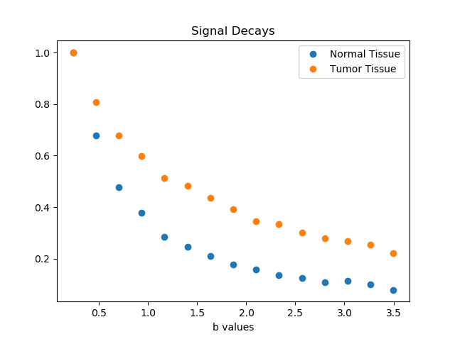
DataDiffusion MRI was performed in men with biopsy proven prostate cancer after obtaining informed consent [5]. Image and signal decay examples are shown in Figs. 1 and 2, respectively.
Spectrum Estimation
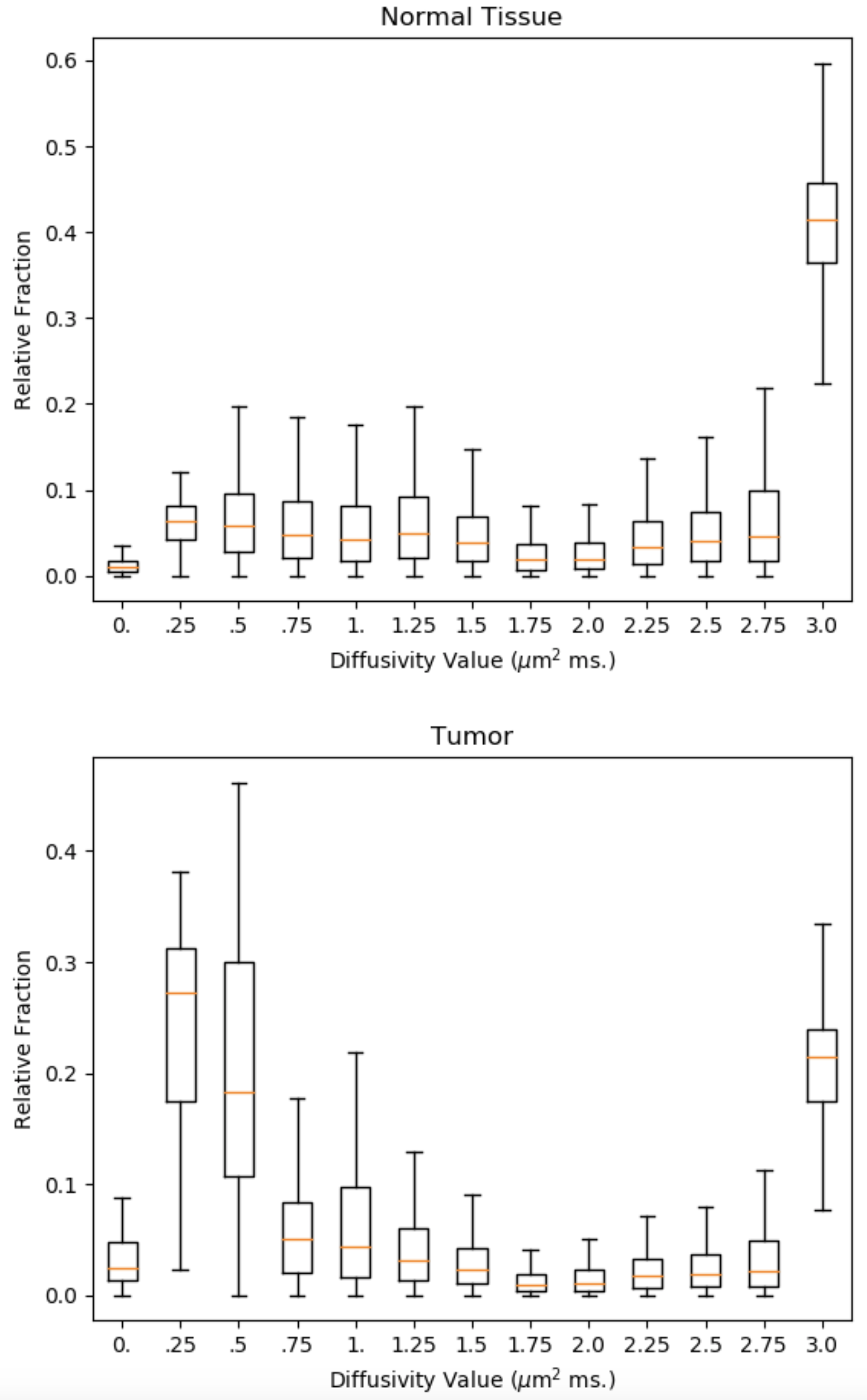
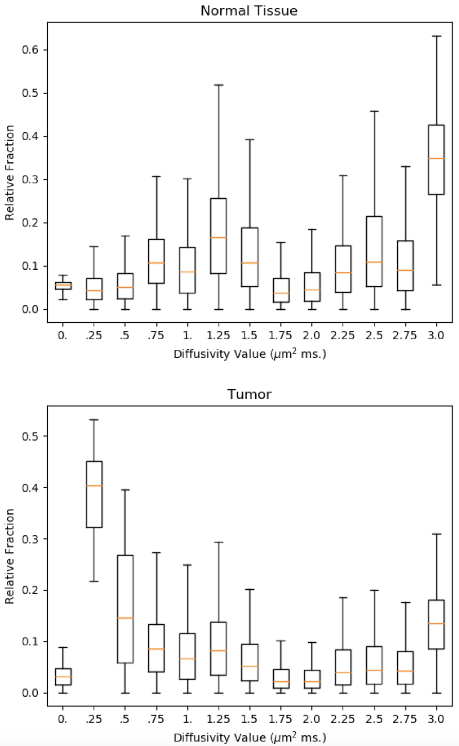
Posterior distributions on relative fractions per diffusivity value were estimated by Gibbs sampling for normal tissue and and tumor data. In consideration that there are no negative diffusivities and that free water diffusion at body temperature equals 3.0 μm$$$^2$$$; diffusivity component values are set to $$$D = [0.0, .25, .5, ..., 3.0]$$$ µm$$$^2$$$ ms; $$$\sigma$$$ was set to $$$1/600$$$. $$$R$$$ was initialized as $$$R^*$$$ and 90k sweeps were sampled after 10k sweeps of burn-in using 52 sec of PC CPU per run. Distributions are summarized by boxplots of samples (Figs. 3 and 4). Mild L2 regularization was used to improve conditioning.
Discussion and Conclusion
While the per-component (vertical) distributions in Figs. 3 and 4 show substantial spread due to limited SNR, there are clear trends. A prominent peak is seen at high diffusivity, corresponding to free water diffusion at body temperature, for both tissue types, but more prominent in normal tissue. The tumor result shows a distinct peak at about .25 μ m$$$^2$$$ ms which agrees very well with dense tissue replacing the lacunar spaces. In normal tissue there is a hint of two moderate peaks for lower diffusivities, which can be interpreted as the glandular and stromal/nuclear compartments [6]. More extensive studies, in a larger number of cases are needed to confirm these preliminary findings. This may also reveal if detected peaks of these diffusivity spectra can aid in the diagnosis of disease. An advantage of this Bayesian approach, over methods such as non-negative least squares, is that, in addition to showing the trends in the data, the Bayes' approach also shows the uncertainty in the result, which can be substantial and important in the interpretation of the results.Related Work
In [5] 5 parametric models of diffusion spectra were analyzed, some on the data treated here. Inverse Laplace transform by nonnegative least squares and related methods have been used in T2 relaxometry from NMR [7] and MRI in [8]. An approach similar to the one we presented here was used to obtain posterior distributions on NMR T2 spectra on synthetic data [9]. As far as we know, the approach presented here has not been used for the analysis of diffusion MRI.
Acknowledgements
This study was supported in part by NIH grants P41EB015902, P41EB028741, and R01CA241817.
References
[1] Mulkern RV, Balasubramanian M, Maier SE. On the perils of multiexponential fitting of diffusion MR data. Journal of Magnetic Resonance Imaging. 2017 May;45(5):1545-7.
[2] Berman P, Levi O, Parmet Y, Saunders M, Wiesman Z. Laplace inversion of low‐resolution NMR relaxometry data using sparse representation methods. Concepts in Magnetic Resonance Part A. 2013 May;42(3):72-88.
[3] Gelman A, Carlin JB, Stern HS, Rubin DB. Bayesian data analysis. Chapman and Hall/CRC; 1995 Jun 1.
[4] Geman S, Geman D. Stochastic relaxation, Gibbs distributions, and the Bayesian restoration of images. IEEE Transactions on pattern analysis and machine intelligence. 1984 Nov(6):721-41.
[5] Langkilde F et al. Evaluation of fitting models for prostate tissue characterization using extended-range b-factor diffusion-weighted imaging. Magn Reson Med. 2018;79(4):2346-2358.
[6] Bourne RM et al. Microscopic diffusivity compartmentation in formalin-fixed prostate tissue. Magn Reson Med. 2012;68:614–620.
[7] Whittall KP, MacKay AL. Quantitative interpretation of NMR relaxation data. Journal of Magnetic Resonance (1969). 1989 Aug 1;84(1):134-52.
[8] Ioannidis, Georgios S., et al. Inverse Laplace transform and multiexponential fitting analysis of T2 relaxometry data: a phantom study with aqueous and fat containing samples. European radiology experimental 4.1 (2020):1-14.
[9] Prange, Michael, and Yi-Qiao Song. Quantifying uncertainty in NMR T2 spectra using Monte Carlo inversion. Journal of Magnetic Resonance 196.1 (2009):54-60.
Figures