Introduction

The diffusion MRI (dMRI) signal can be mathematically described via the cumulant expansion, yielding the commonly used DTI and DKI methods. Conventional linear tensor encoding (LTE) allows measuring the kurtosis tensor $$$\boldsymbol{W}$$$¹ with 15 independent components. However, dMRI protocols adding free (beyond LTE) $$$q$$$-space trajectories² enable probing a more general diffusion covariance tensor $$$\boldsymbol{C}$$$³ with 21 independent components. Here we characterize and explore the information content of $$$\boldsymbol{C}$$$. We represent the $$$6=21-15$$$ extra parameters in terms of a rank-2 symmetric tensor $$$\boldsymbol{A}$$$, and construct its rotational invariants $$$A_0$$$ and $$$A_2$$$. While $$$A_0$$$ contributes to microscopic fractional anisotropy ($$$\mu$$$FA), the previously unexplored invariant $$$A_2$$$ yields the size-shape covariance of the compartmental diffusivities over a voxel. We measure all rotational invariants of $$$\boldsymbol{W}$$$ and $$$\boldsymbol{A}$$$ in a normal volunteer, explore the novel size-shape contrast, and show how to calculate axial and radial kurtosis metrics fast, without projecting the tensors onto a principal fiber direction.

Theory

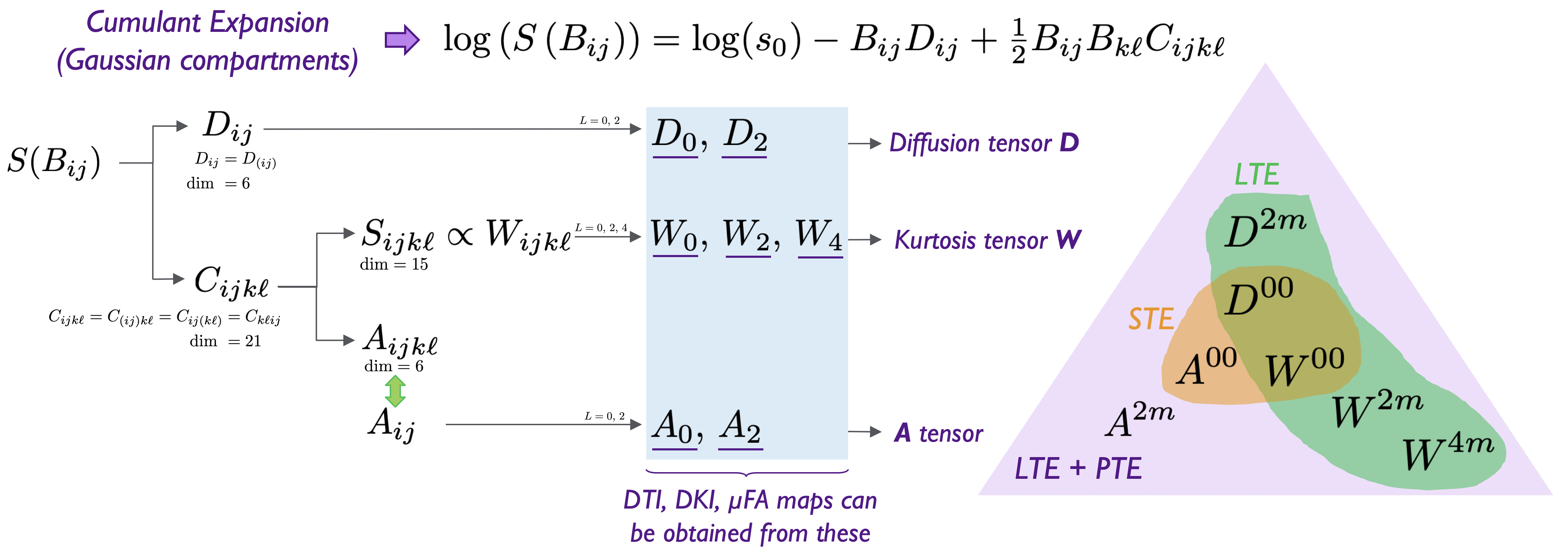
Cumulant expansion. If a voxel contains multiple Gaussian compartments, the signal from any q-space trajectory, $$$\boldsymbol{q}(t)$$$, is fully determined by a b-tensor $$$\boldsymbol{B}$$$³:$$\begin{aligned}S&=s_0\sum_\alpha\,f_\alpha\,e^{-B_{ij}D_{ij}^\alpha},\qquad(1)\\B_{ij}&=\int_0^{\text{TE}}\!\!q_i(t)\,q_j(t)\,\mathrm{d}t,\qquad(2)\end{aligned}$$where $$$D_{ij}^\alpha$$$ is the diffusion tensor of compartment $$$\alpha$$$ and $$$b=B_{ii}=\mathrm{tr}\,\boldsymbol{B}$$$ is the b-value (Einstein's convention of summation over repeated indices assumed).
We can write the cumulant expansion of Eq. 1 up to $$$\mathcal{O}(B^2)$$$:$$\log(S)=\log(s_0)-B_{ij}\,D_{ij}+\tfrac12B_{ij}B_{k\ell}C_{ijk\ell},\qquad(3)$$where $$$\boldsymbol{D}$$$ and $$$\boldsymbol{C}$$$ are the diffusion and covariance tensors, determined by:$$D_{ij}=\langle\,\!D_{ij}^\alpha\rangle,\,\,\,C_{ijk\ell}=\langle\,\!D_{ij}^\alpha\,D_{k\ell}^\alpha\rangle-\langle\,\!D_{ij}^\alpha\rangle\,\langle\,\!D_{k\ell}^\alpha\rangle,\qquad(4)$$with angular brackets denoting averages over the distribution of $$$D_{ij}^\alpha$$$ in a voxel. $$$\boldsymbol{C}$$$ has minor and major symmetries and can be decomposed into its symmetric part, $$$\boldsymbol{S}$$$, and its complement, $$$\boldsymbol{A}$$$:⁴
$$\begin{aligned}C_{ijk\ell}&=S_{ijk\ell}+A_{ijk\ell},\\S_{ijk\ell}&=C_{(ijk\ell)}=\tfrac13(C_{ijk\ell}+2C_{i\ell\,\!kj}),\quad\quad\quad\quad(5)\\A_{ijk\ell}&=C_{ijk\ell}-C_{(ijk\ell)}=\tfrac23(C_{ijk\ell}-C_{i\ell\,\!kj}).\end{aligned}$$Here symmetrization over tensor indices between (...) is assumed.
Tensor $$$\boldsymbol{S}$$$ is accessible with LTE, it has 15 degrees of freedom (dof) and is proportional to the kurtosis tensor: $$$W_{ijk\ell}=\frac{3}{\overline{D}^2}C_{(ijk\ell)}=\frac{3}{\overline{D}^2}S_{ijk\ell}$$$, where $$$\overline{D}$$$ is mean diffusivity.
Tensor $$$\boldsymbol{A}$$$, inaccessible with LTE, has 6 dof which can be mapped to a rank-2 symmetric tensor⁴:$$\begin{aligned}A_{mn}&=\epsilon_{ikm}\epsilon_{j\ell\,\!n}A_{ijk\ell}=\delta_{mn}(A_{iikk}-A_{ikik})+2A_{mknk}-2A_{mnkk}=\delta_{mn}(C_{iikk}-C_{ikik})+2C_{mknk}-2C_{mnkk},\qquad(6)\\A_{ijk\ell}&=\tfrac16(\epsilon_{ikm}\epsilon_{j\ell\,\!n}+\epsilon_{i\ell\,\!m}\epsilon_{jkn})A_{mn},\end{aligned}$$where $$$\delta_{ij}$$$ is Kronecker's delta, and $$$\epsilon_{ijk}$$$ the Levi-Civita symbol. Spherical tensor encoding (STE) is sensitive to the isotropic part of $$$\boldsymbol{A}$$$ while planar tensor encoding (PTE) probes the full $$$\boldsymbol{A}$$$ tensor. Figure 1 shows a diagram of this decomposition.

STF decompositions. We represent voxel-wise tensors $$$\boldsymbol{D}$$$, $$$\boldsymbol{S}$$$ and $$$\boldsymbol{A}$$$ in STF basis $$$\mathcal{Y}_{i_1...i_\ell}^{\ell\,\!m}$$$⁵:$$\begin{aligned}D_{ij}&=D_{00}\tfrac{1}{\sqrt{4\pi}}\delta_{ij}+D_{2m}\mathcal{Y}_{ij}^{2m},\\S_{ijk\ell}&=S_{00}\tfrac{1}{\sqrt{4\pi}}\delta_{(ij}\delta_{k\ell)}+S_{2m}\mathcal{Y}_{(ij}^{2m}\delta_{k\ell)}+S_{4m}\mathcal{Y}_{ijk\ell}^{4m},\qquad(7)\\A_{ij}&=A_{00}\tfrac{1}{\sqrt{4\pi}}\delta_{ij}+A_{2m}\mathcal{Y}_{ij}^{2m}.\end{aligned}$$This basis is analogous to spherical harmonics. For every order $$$\ell$$$ we can define rotational invariants^6,7,8, e.g. $$$S_\ell=\sqrt{\frac{\sum_m|S_{\ell\,\!m}|^2}{4\pi(2\ell+1)}}$$$.
Writing compartmental diffusion tensors in STF basis, $$$D_{ij}^\alpha=D_{00}^\alpha\tfrac{1}{\sqrt{4\pi}}\delta_{ij}+D_{2m}^\alpha\mathcal{Y}_{ij}^{2m}$$$, we derive all terms in Equation 7 averaged over arbitrary distribution of compartmental $$$D_{ij}^\alpha$$$:$$L=0\quad\left\{\begin{aligned}D_0=&\,\langle\,\!D_0^\alpha\rangle\\S_0=&\,\langle(D_0^\alpha)^2\rangle-D_0^2+5\big(\,\langle(D_2^\alpha)^2\rangle-D_2^2\big)\qquad(8)\\A_0=&\,2\big(\,\langle(D_0^\alpha)^2\rangle-D_0^2\big)-\tfrac{25}{2}\big(\,\langle(D_2^\alpha)^2\rangle-D_2^2\big)\end{aligned}\right.$$ $$L=2\quad\left\{\begin{aligned}D_{2m}=&\,\langle\,\!D_{2m}^\alpha\rangle\\S_{2m}=&\,2\,(\,\langle\,\!D_0^\alpha\,D_{2m}^\alpha\rangle-D_0\,D_{2m})+\tfrac{8}{21C_2^2}\,(\langle\,\!D_{2m'}^\alpha\,D_{2n'}^\alpha\rangle-D_{2m'}\,D_{2n'})\,\mathcal{Y}^{2m'}_{ij}\,\mathcal{Y}^{2n'}_{jk}\mathcal{Y}^{2m}_{ki}\qquad(9)\\A_{2m}=&\,-2\,(\,\langle\,\!D_0^\alpha\,D_{2m}^\alpha\rangle-D_0\,D_{2m})+\tfrac{4}{3C_2^2}\,(\langle\,\!D_{2m'}^\alpha\,D_{2n'}^\alpha\rangle-D_{2m'}\,D_{2n'})\,\mathcal{Y}^{2m'}_{ij}\,\mathcal{Y}^{2n'}_{jk}\mathcal{Y}^{2m}_{ki}\end{aligned}\right.$$ $$L=4\quad\left\{\begin{aligned}S_{4m}=&\,\tfrac{8}{35C_4^2}\,(\langle\,\!D_{2m'}^\alpha\,D_{2n'}^\alpha\rangle-D_{2m'}\,D_{2n'})\,\mathcal{Y}^{4m}_{ijk\ell}\,\mathcal{Y}^{2m'}_{(ij}\mathcal{Y}^{2n'}_{k\ell)}.\qquad(10)\end{aligned}\right.$$

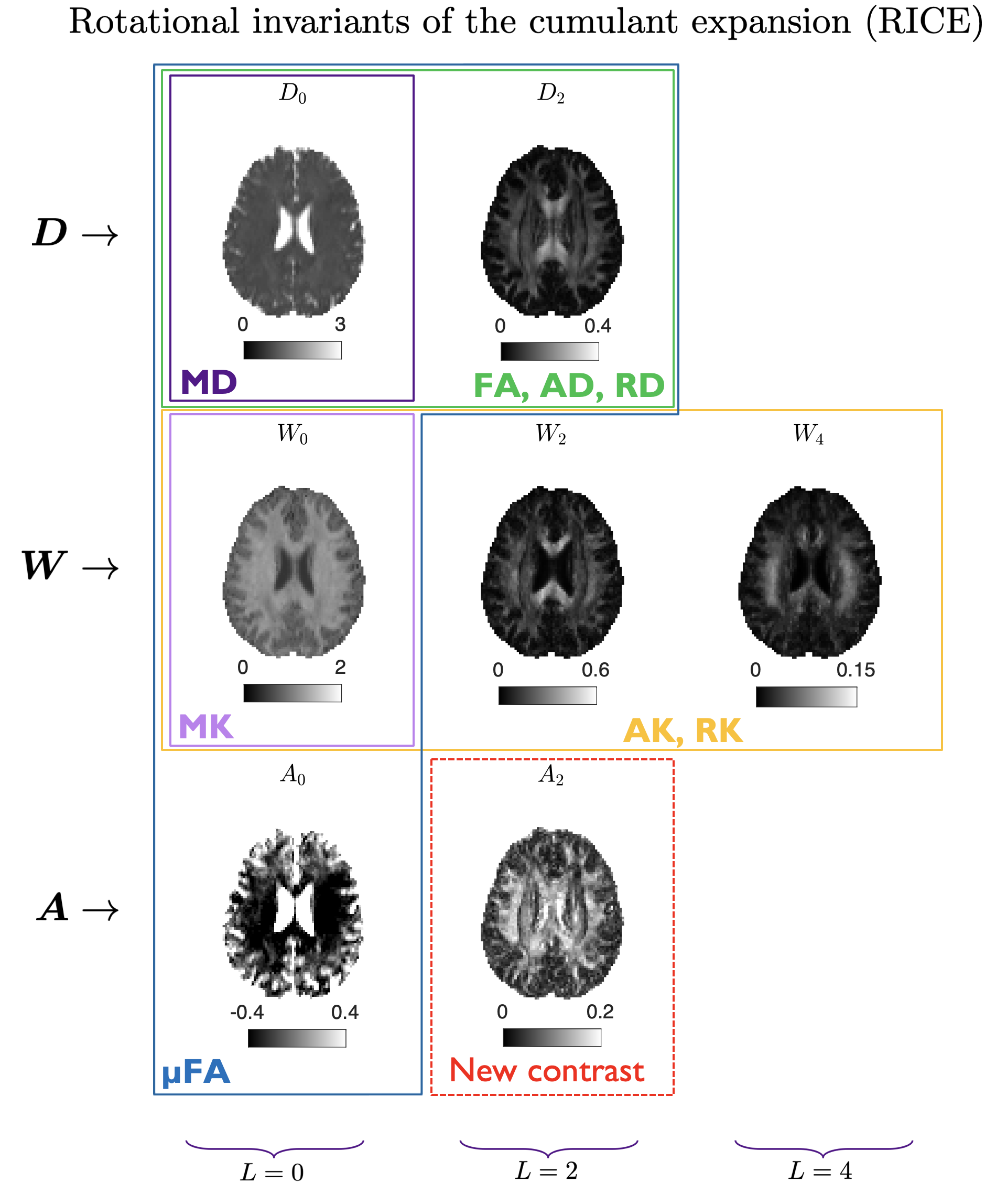
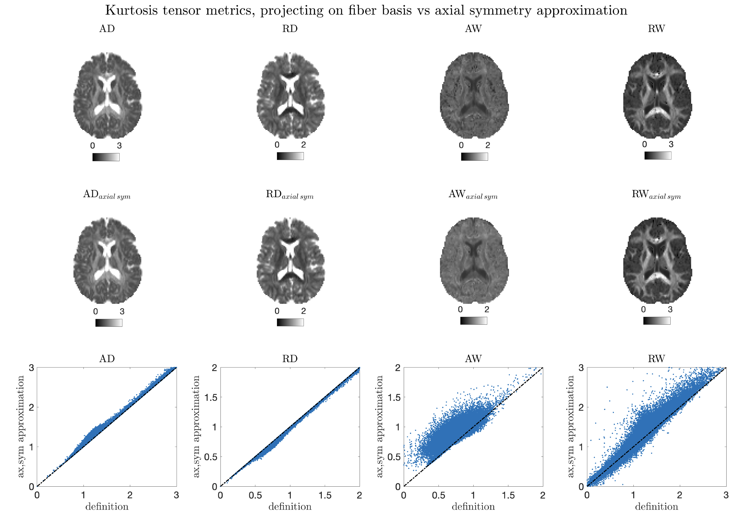
Conventional contrasts. We can derive DTI maps from RICE:$$\begin{aligned}\text{MD}&=\overline{D}=\tfrac{1}{4\pi}\int_{\mathbb{S}^2}d\hat{\boldsymbol{n}}D(\hat{\boldsymbol{n}})=\tfrac13\delta_{ij}D_{ij}=\tfrac{1}{\sqrt{4\pi}}D_{00}=D_0,\qquad(11)\\\text{FA}^2&=\frac32\frac{{V_{\lambda}(\boldsymbol{D})}}{{V_{\lambda}(\boldsymbol{D})}+3\overline{D}^{2}}=\frac{75D_2^2}{4D_0^2+50D_2^2},\qquad(12)\end{aligned}$$where $$$V_{\lambda}(\boldsymbol{D})$$$ is the variance of the eigenvalues of $$$\boldsymbol{D}$$$. For kurtosis, we use tensor derived metrics rather than average apparent kurtosis^6,9,10:$$\text{MK}=\overline{W}=\tfrac{1}{4\pi}\int_{\mathbb{S}^2}d\hat{\boldsymbol{n}}W(\hat{\boldsymbol{n}})=\tfrac15\delta_{ij}\delta_{k\ell}W_{ijk\ell}=\tfrac{1}{\sqrt{4\pi}}W_{00}=W_0.\qquad(13)$$Often a main fiber population is assumed, thus, $$$\boldsymbol{D}$$$ and $$$\boldsymbol{W}$$$ can be projected to this principal axis $$$\hat{\boldsymbol{v}}_1$$$:$$\begin{aligned}\text{AD}&=D_\|=D(\hat{\boldsymbol{v}}_1),\quad &&\text{RD}=D_\perp=\tfrac{1}{2\pi}\int_{\mathbb{S}^2}d\hat{\boldsymbol{n}}D(\hat{\boldsymbol{n}})\delta(\hat{\boldsymbol{n}}\cdot\hat{\boldsymbol{v}}_1),\qquad(14)\\\text{AK}&=W_\|=\frac{\overline{D}^2}{D_\|^2}\,W(\hat{\boldsymbol{v}}_1),&&\text{RK}=W_\perp=\frac{\overline{D}^2}{D_\perp^2}\,\tfrac{1}{2\pi}\int_{\mathbb{S}^2}d\hat{\boldsymbol{n}}W(\hat{\boldsymbol{n}})\delta(\hat{\boldsymbol{n}}\cdot\hat{\boldsymbol{v}}_1).\end{aligned}$$Note that if $$$\boldsymbol{D}$$$ and $$$\boldsymbol{W}$$$ possess axial symmetry, we can compute the above maps without projecting onto the fiber basis but directly from RICE maps:$$\begin{aligned}\text{AD}_\text{ax,sym}&=D_0+5D_2,\quad&&\text{RD}_\text{ax,sym}=D_0-\tfrac52D_2\qquad\qquad\qquad\qquad(15)\\\text{AK}_\text{ax,sym}&=\frac{\overline{D}^2}{D_\|^2}\,(W_0+5W_2+9W_4),\quad&&\text{RK}_\text{ax,sym}=\frac{\overline{D}^2}{D_\perp^2}\,(W_0-\tfrac52W_2+\tfrac{27}{8}W_4).\end{aligned}$$Extracting the shape variance, $$$\langle(D_2^\alpha)^2\rangle$$$, we can compute $$$\mu$$$FA^3,11
$$\mu\text{FA}^{2}=\frac32\frac{\langle\,\!V_{\lambda}(\boldsymbol{D})\rangle}{\langle\,\!V_{\lambda}(\boldsymbol{D})\rangle+3\overline{D}^{2}}=\frac{75\langle(D_2^\alpha)^2\rangle}{4D_{0}^{2}+50\langle(D_2^\alpha)^2\rangle}=\frac{60(S_0-\tfrac12A_0)+675D_2^2}{40(S_0-\tfrac12A_0)+450D_2^2+36D_0^2}.\qquad(16)$$

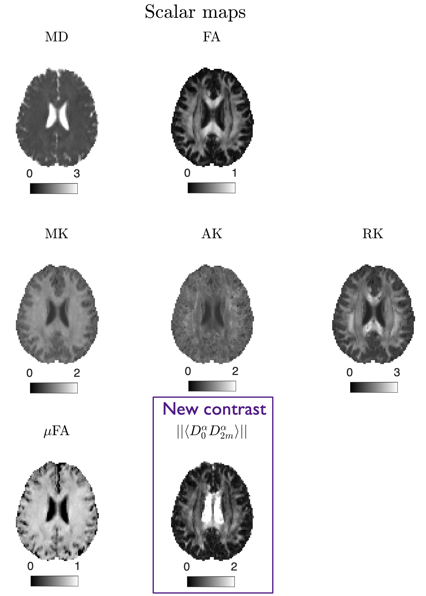
Novel contrast. All maps above are independent of $$$A_{2m}$$$ elements, which contain previously unexplored information. Following Eq. 9, we can obtain size-shape covariances and compute an invariant that is complementary to DTI-DKI-$$$\mu$$$FA:$$\langle\,\!D_0^\alpha\,D_{2m}^\alpha\rangle=\tfrac{7}{18}S_{2m}-\tfrac19A_{2m}+D_0D_{2m},\quad\rightarrow\quad||\langle\,\!D_0^\alpha\,D_{2m}^\alpha\rangle||=\sqrt{\sum_{m=-2}^{2}\langle\,\!D_0^\alpha\,D_{2m}^\alpha\rangle^2}.\qquad(17)$$

Experiments

After providing inform consent, a 30yo female volunteer underwent MRI in a whole body 3T-system (Siemens Healthcare, Prisma) using a 20-channel head coil. Maxwell-compensated free gradient diffusion waveforms were used to yield linear, planar, and spherical b-tensor encoding using a prototype spin echo sequence with EPI readout¹². Linear b-tensors (30 directions $$$b=1ms/\mu\,\!m^2$$$ + 60 directions $$$b=2ms/\mu\,\!m^2$$$) and planar b-tensors (60 directions $$$b=1.5ms/\mu\,\!m^2$$$) were acquired. Imaging parameters: voxel size$$$\,=2\times2\times2\,$$$mm$$$^3$$$, $$$T_R=4.2s$$$, $$$T_E=90$$$ms, bandwidth=1818Hz/Px, $$$R_\text{GRAPPA}=2$$$, partial Fourier$$$\,=6/8$$$, multiband$$$\,=2$$$. Total scan was time 11.5 minutes.

Results

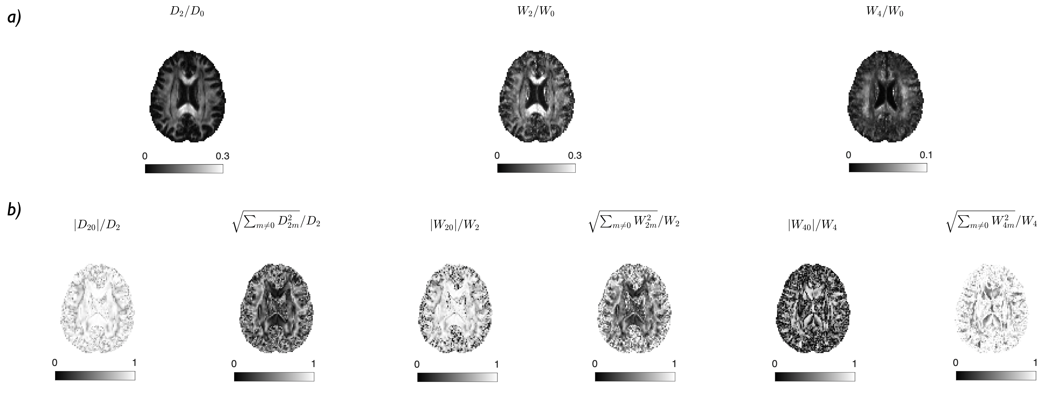
All rotational invariants of the cumulant expansion (RICE) maps are shown in Fig. 2. Figure 3 shows conventional diffusion contrasts together with a $$$||\langle\,\!D_0^\alpha\,D_{2m}^\alpha\rangle||$$$ map that contains the proposed size-shape covariance. The relative contributions from $$$L=0,2,4$$$ sectors in $$$\boldsymbol{D}$$$ and $$$\boldsymbol{W}$$$ are analyzed and shown in Fig. 4. Furthermore, we rotate each voxel and separate the contributions of the main axis vs the rest ($$$m=0\,\text{vs}\,m\neq0$$$ at the fiber coordinate frame). Finally, a comparison between fiber-basis projection maps (axial and radial diffusion/kurtosis) and axial symmetry approximations is shown in Fig. 5.

Discussion and Conclusion

We classified the symmetries of the full diffusion covariance tensor $$$\boldsymbol{C}$$$ accessible under a general diffusion tensor-encoding acquisition. We showed that there is an unexplored contrast in the non-symmetric part of $$$\boldsymbol{C}$$$, and related it to the size-shape covariance of compartmental diffusion tensors. The RICE maps belong to distinct irreducible representations of rotations and thereby represent the ``orthogonal" contrasts up to $$$B^2$$$. This mutual independence may provide improved sensitivity to detect independent changes in disease and development.

Acknowledgements

This work has been supported by NIH under NINDS award R01 NS088040 and NIBIB awards R01 EB027075 and P41 EB017183. The authors are grateful to Sune N. Jespersen for fruitful discussions.