Introduction

Quantitative MRI at 7T may have important clinical applications owing to enhanced resolution and the potential for uniform tissue characterization. However, optimizing protocols to achieve precise parameter mapping across the whole brain with high resolution remains challenging, particularly due to large variability in transmit field (B₁+). In this abstract, we aimed to validate the Cramer-Rao Lower Bound (CRLB) approach to optimize T₁ mapping for a dual flip angle SPGR acquisition in the context of B₁ inhomogeneity. Validation was performed in simulations, phantom and in vivo.

Methods

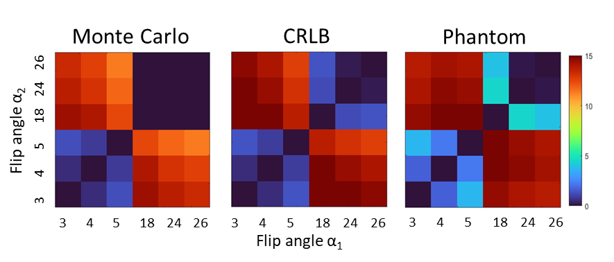
All simulations were performed in MATLAB 2021b (www.mathworks.com).

Monte Carlo simulation: A spoiled gradient echo sequence (SPGR) was simulated as a function of longitudinal relaxation time (T₁), flip-angle (α), transmit B₁ bias factor (κ), equilibrium magnetization (M0) using the Ernst equation [1] assuming perfect spoiling and a steady state. Signals were obtained with α=3°,4°..,26° and 100,000 instances of gaussian noise (σ=0.001) were added. Variance in T1 estimation was calculated for each possible combination of SPGR signals {Si(αi), Sj(αj)} such that {αi,αj}∈α. CRLB simulation: Based on the framework [2], the T₁ parameter precision estimate was calculated for the same set of α ‘s and same gaussian noise (σ=0.001) was assumed.

A first set of simulations (CRLB and Monte Carlo) were performed with TR=20ms and a set of T₁s corresponding to phantom values: T₁s= 440ms, 550ms, 760ms, 1200ms, 2200ms and M0=1.0 (a.u.) assuming no B₁(+) variability. The worst case variance was obtained as a 2D grid corresponding to the two flip angles. The normalized inverse of this variance was used as a measure of precision for each {αi, αj} with the peak value being the optimal. A second simulation was performed (CRLB only) with a TR=20ms and T₁=1200ms, 2130ms [3] and M0 = 0.69,0.82 corresponding to 7T brain white matter and gray matter values. Here, B₁(+) variability was incorporated by summing the worst-case variances calculated with κ∈{0.46, 0.63, 0.8, 0.97, 1.14} corresponding to the B₁(+) map.

Experimental validation of the simulations was performed using a 120mm diameter cylindrical phantom, length 137mm, (Gold Standards Phantoms) containing eight equally-spaced test tubes filled with varying concentrations of MnCl2 (0.01mM, 0.05 mM, 0.1mM, 0.15 mM, 0.2 mM) and the remaining space was filled with rapeseed oil in order to minimize the B₁(+) variability. B₁(+) field homogeneity was mapped using the actual flip angle imaging method with αnom=50° [4]. The T1 and PD values of each solution was determined using a conventional long-TR 2D inversion recovery experiment [5] at multiple TI times (100,200..,3000ms). Images were obtained with a 6-echo SPGR protocol (0.6mm isotropic, TR=20ms) for α’s = 3°,4°,5°,18°,24° and 26°. Only the first image (TE=2.4ms) was used further. ROIs around each test-tube were obtained using imfindcircles.m and imerode.m functions, removing outer voxels compromised by fat-water shifts. T₁ was estimated for each possible {αi, αj} using a linearized approximation of Ernst equation at short TR and low flip angles [6]. The corresponding precision heatmap was calculated to measure the optimal flip angles.

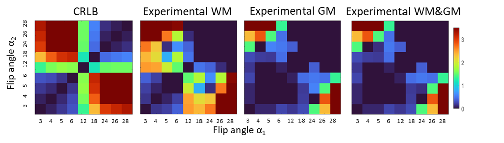
Using the same SPGR acquisition protocol (but 1mm isotropic resolution), in vivo data was acquired from a healthy volunteer adult at a TR = 20ms for α’s = 3°,4°,5°,6°,12°,18°,24°,26°and 28°. The SPGR images were coregistered and segmented using spm12. T₁ was estimated for each possible pair of SPGR images and the normalized precision was calculated for each tissue.

Results

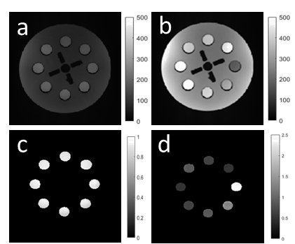
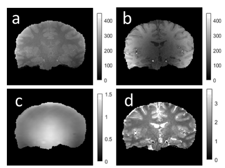
The results of the simulations and phantom validation are shown in Fig. 1 which depicts the T₁ precision heatmap for different flip angles pairs {αi,αj} and phantom T₁ range. The optimal flip angles from both simulations were consistently found to be 3° & 18° while experimental results in the phantom were 4° & 18°. Fig.2(a-b) shows representative phantom SPGR images for flip angles 4° and 18°, residual B₁(+) correction map in Fig. 2(c) and the T₁ map in Fig. 2(d).

The results of optimization for human brain T₁ precision using the CRLB simulation are shown in Fig. 3 together with in-vivo white matter, gray matter and combined precision. The optimal flip angles from the simulation were 4° and 26°, while experimental optimal flip angles were 4° and 28°. Fig.4(a-b) shows representative in-vivo SPGR images for flip angles 4° and 28° with the B₁(+) map in Fig4(c) and the T₁ map shown in Fig. 4(d).

Discussion

In this abstract, we showed a method to minimize the parameter estimate variance and obtain the optimal flip angles for quantitative T₁ mapping using Monte Carlo and CRLB calculation. We validated simulation results by measuring T₁ precision in a phantom and in vivo in the context of B₁(+) variability. Modest discrepancies in the T₁ precision map for in vivo data may be due to the way in which B₁(+) distribution across the whole brain were accounted for in the simulation. Error in the B₁(+) field mapping [7] may offer an alternative explanation. The CRLB approach provides a framework that can be extended to optimize multiple sequence parameters (e.g. TR and TE) and parameter maps (e.g. T₂* and PD) to maximize precision for the development of more complex mapping protocols.

References

- Ernst, R. R., and Anderson W. A. (1966), Application of Fourier Transform Spectroscopy to Magnetic Resonance, Review of Scientific Instruments 37, 93-102
- Teixeira, R.P.A., Malik, S.J. and Hajnal, J.V. (2018), Joint system relaxometry (JSR) and Crámer-Rao lower bound optimization of sequence parameters: A framework for enhanced precision of DESPOT T1 and T2 estimation, Magn. Reson. Med, 79: 234-245
- Wright, P.J., Mougin, O.E., Totman, J.J. et al. (2008), Water proton T1 measurements in brain tissue at 7, 3, and 1.5T using IR-EPI, IR-TSE, and MPRAGE: results and optimization, Magn Reson Mater Phy 21, 121
- Yarnykh VL. (2007), Actual flip-angle imaging in the pulsed steady state: a method for rapid three-dimensional mapping of the transmitted radiofrequency field, Magn Reson Med.;57(1):192-200
- Kleinberg R., Encyclopedia of Nuclear Magnetic Resonance, Wiley; New York, USA: 1995
- Helms, G., Dathe, H. and Dechent, P. (2008), Quantitative FLASH MRI at 3T using a rational approximation of the Ernst equation, Magn. Reson. Med., 59: 667-672
- Olsson H., Andersen M., Helms G., (2020) Reducing bias in DREAM flip angle mapping in human brain at 7T by multiple preparation flip angles, Magn. Reson. Imaging, 72, 71-77