Purpose

To evaluate the correlations between various quantitative maps derived from different diffusion MRI models and 3D Nissl staining of whole mouse brain at microscopic resolution.

Introduction

Diffusion MRI (dMRI) affords unique image contrasts and has gained prominence to non-destructively probe the tissue microstructure, validation the MRI findings with conventional histology is essential for better understanding the original of MRI signal (1,2). However, dMRI often suffers from relatively low spatial resolution due to its inherently low signal-to-noise ratio (SNR) and long scan time, which impedes the accurate comparison between quantitative dMRI metrics and traditional histology (3,4). In this study, we acquired high angular and high spatial resolution whole mouse brain diffusion MRI dataset with the b value from 1000 to 8000 s/mm², quantitative parameters from different dMRI models have been generated and compared with 3D whole brain Nissl staining.

Methods

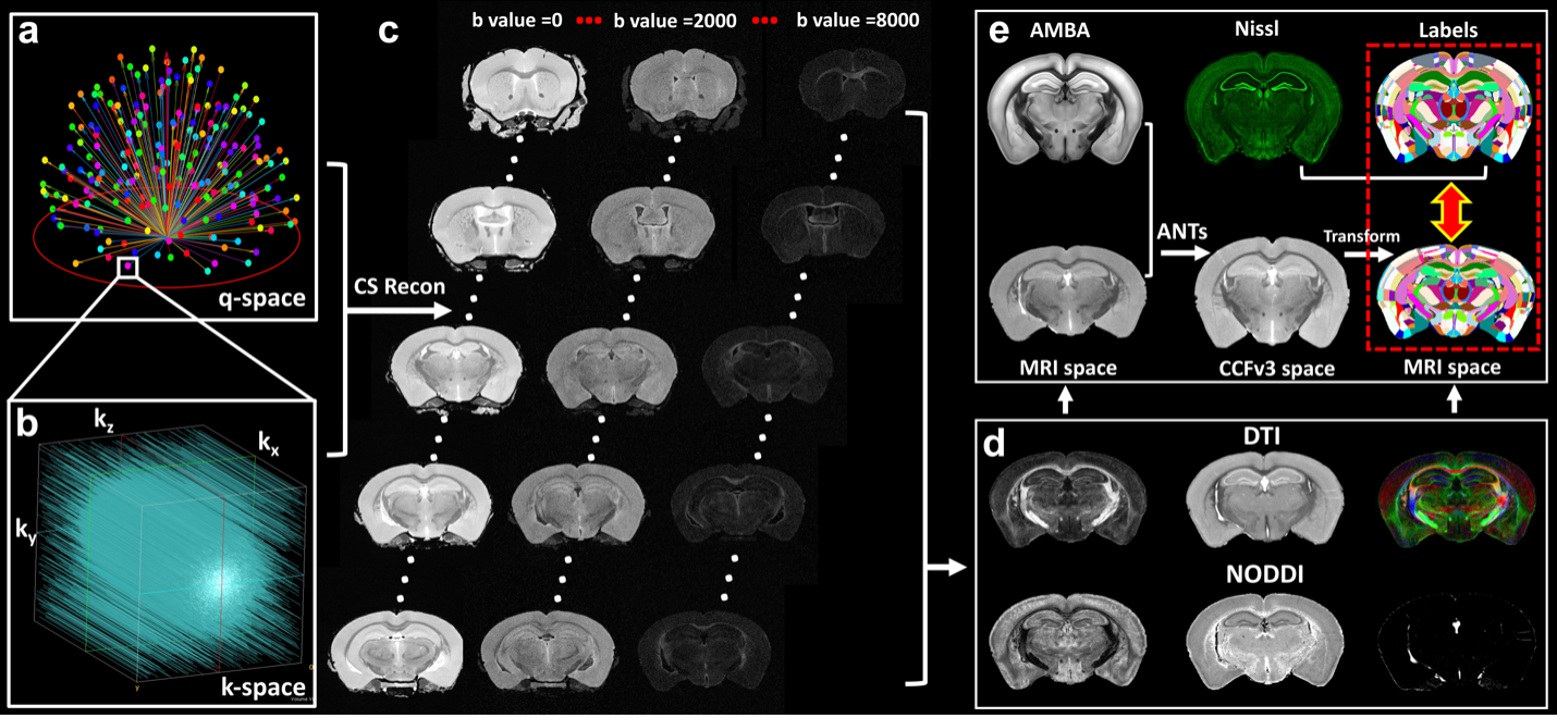
Animal experiments were carried out in compliance with the local IACUC Committee. Wild-type C57BL/6 mice (Jackson Laboratory, Bar Harbor, ME) were chosen for brain imaging. Animals were sacrificed and perfusion fixed with a 1:10 mixture of ProHance-buffered (Bracco Diagnostics, Princeton, NJ) formalin to shorten T1 and reduce scan time. The specimens were scanned at 9.4 T (Oxford 8.9-cm vertical bore) with maximum gradient strength of 2000 mT/m on each axis using a modified 3D Stejskal-Tanner diffusion-weighted (DW) spin-echo pulse sequence (5). The dMRI dataset was axquired with multiple shells (b value = 1000, 2000, 3000, 4000, 5000, 6000, 7000, 8000 s/mm²) at 25 μm isotropic resolution. The total scan time was approximately 213 hours (~ 0.91 hours/volume) with 216 DWIs and 18 b0 images. The repetition time (TR) was 100 ms and the TE was15.2 ms. The gradient separation time was 7.7 ms, and the diffusion gradient duration time was 4.8 ms. The DTI model and NODDI model were used to calculate the quantitative maps (6,7). The images were registered to Allen Mouse Brain Atlas (AMBA) in the Allen mouse brain common coordinate framework (CCFv3) using Advanced Normalization Tools (ANTs).

Results

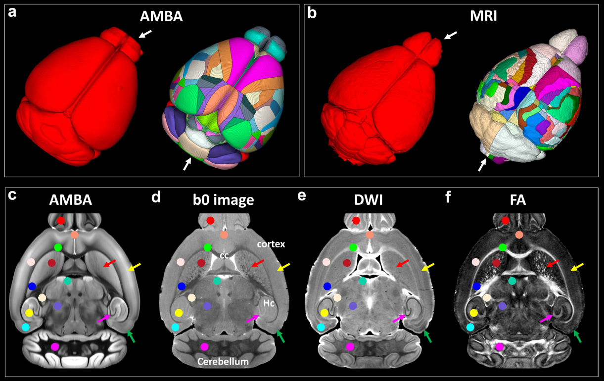
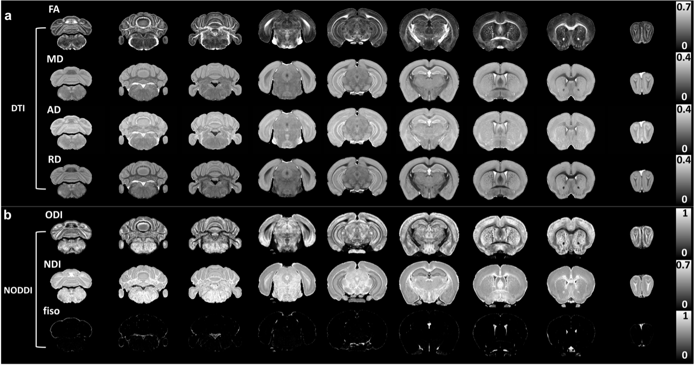
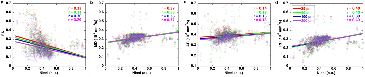
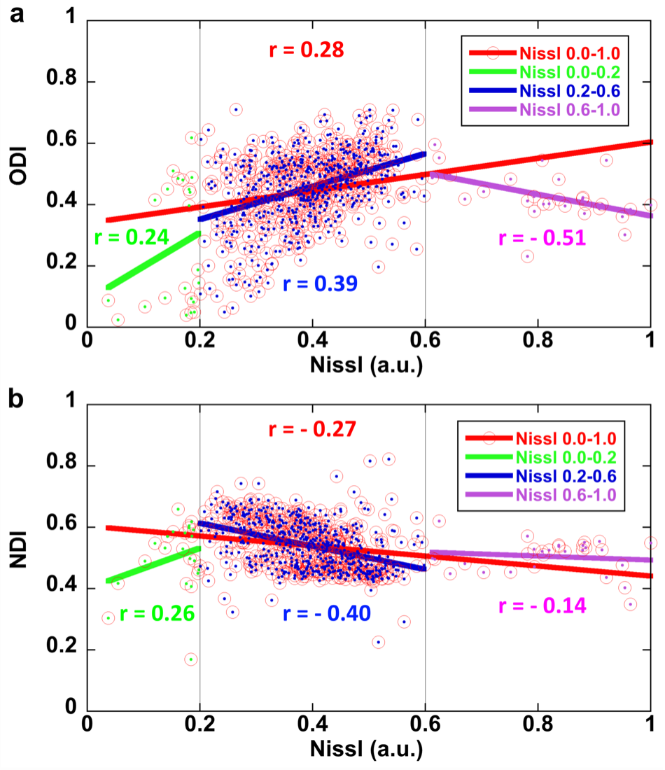
Figure 1 shows a summary of the methods used in this study from data acquisition to the imaging reconstruction and analysis. The individual slices of each 3D DWI volume were reconstructed using a nonlinear iterative reconstruction. The MRI images were registered to CCFv3 space. The labels of the AMBA were transformed back to MRI space for ROI-based analysis. Figure 2 shows a comparison between the AMBA in CCFv3 space and the dMRI atlas. The MRI images were registered to AMBA for a side-by-side comparison and the registration accuracy was visualized using the manual landmarks (dots in different colors). The representative slices of quantitative dMRI maps from both DTI and NODDI models are shown in Figure 3, where each map demonstrated unique image contrast. FA and ODI exhibited opposite contrast, where higher ODI regions showed lower FA values. The similar inverse contrast was also found between NDI and MD maps. Compared to AD, the RD showed lower values in white matter regions. The correlation between Nissl staining intensity and DTI metrics at different spatial resolution (25 µm to 200 µm) throughout the whole mouse brain are shown in Figure 4. Compared to FA (r ranging from 0. 29 to 0.33), MD (r ranging from 0.36 to 0.38) and RD (r ranging from 0.39 to 0.40) showed relatively higher correlation with Nissl staining. In contrast, the correlation between AD and Nissl staining was relatively low (ranging from 0.14 to 0.18). The correlation between Nissl staining intensity and NODDI metrics (ODI and NDI) at 25 µm resolution are illustrated in Figure 5. The ODI (r = 0.28) showed a slightly lower correlation coefficient compared to that of FA (r = 0.33); the NDI (r = 0.27) showed a lower correlation coefficient compared to that of MD (r = 0.37). To explore whether the correlation was also dependent on the Nissl staining intensity, we divided the Nissl staining intensity into the following 3 levels: low intensity regions (intensity between 0.0 to 0.2), medium intensity regions (intensity between 0.2 to 0.6), and high intensity regions (between 0.6 to 1.0). The ODI showed a higher negative correlation at high intensity regions (r = - 0.51), and the NDI showed a higher negative correlation at medium intensity regions (r = -0.40).

Discussion and Conclusion

We integrated dMRI datasets at microscopic resolution to the CCFv3 space, which provide an opportunity to visualize the fine neuroanatomy of the mouse brain with different imaging modalities at the same spatial resolution and at the same common space. This approach also allowed us to quantitatively compare different dMRI parameters with 3D Nissl staining throughout the whole brain. Each dMRI metric exhibited a unique image contrast and showed a different correlation coefficient to the Nissl staining. The unique imaging contrasts provided by quantitative dMRI maps in cerebellum and hippocampus may not be captured by Nissl staining. Developing advanced dMRI models with high specificity is essential to improve the correlation between MRI and histology results in future studies.

Acknowledgements

This work was supported by NIH/NIBIB P41 EB015897, and Charles E. Putman MD Vision Award of the Department of Radiology, Duke University School of Medicine.