0683
Accelerating High b-Value DWI Acquisition Using a Convolutional Recurrent Neural Network1Radiology, Stanford University, Stanford, CA, United States, 2Homestead High School, Cupertino, CA, United States, 3Center for MR Research, University of Illinois at Chicago, Chicago, IL, United States, 4Radiology, Neurosurgery and Bioengineering, University of Illinois at Chicago, Chicago, IL, United States
Synopsis
DWI can probe tissue microstructures in many disease processes over a broad range of b-values. In the scenario where severe geometric distortion presents, non-single-shot EPI techniques can be used, but introduce other issues such as lengthened acquisition times, which often requires undersampling in kspace. Deep learning has been demonstrated to achieve many-fold undersampling especially when highly redundant information is present. In this study, we have applied a novel convolutional recurrent neural network (CRNN) to reconstruct highly undersampled (up to six-fold) multi-b-value, multi-direction DWI dataset by exploiting the information redundancy in the multiple b-values and diffusion gradient directions.
Introduction
Diffusion-weighted imaging (DWI) can probe tissue microstructural alterations in many disease processes, which has been demonstrated over a broad range of b-values with different diffusion models1–5. The widely used sequence in DWI – single-shot EPI – is subject to geometric distortion despite its rapid scan speed and resilience to motion. Multi-shot sequences have been proposed to mitigate this problem. However, they often prolong the acquisition times and/or accentuate the SAR issue6. An alternative strategy is to substantially undersample k-space data, as in parallel imaging and recently emerging deep learning techniques7,8. Among the many deep learning neural networks, a convolutional recurrent neural network (CRNN)9 is of particular interest because it combines convolutional neural network (CNN) and recurrent neural network (RNN), thereby providing better image quality through exploiting spatio-temporal redundancy in a series of images, such as the time series in dynamic imaging. Recognizing that the image series can be generalized to a set of diffusion images with different b-value and/or different diffusion directions, we hypothesize that the CRNN approach can be applied to reconstructing highly undersampled multi-b-value DWI data. Herein, we employ a novel neural network – CRNN-DWI – and demonstrate its ability to achieve up to six-fold undersampling in DWI without degrading the image quality.Methods
CRNN-DWI:Multi-b-value DWI series exhibit similar image features (i.e., edges, anatomy) among differing b-values and diffusion directions (Figure 1). Exploiting this information in a neural network can effectively train it to reconstruct highly undersampled k-space data. The formulation of the proposed CRNN-DWI is expressed as:
$$X_{rec}=f_{N}(f_{N-1}(...(f_{1}(X_{u})))), (1)$$
where $$$X_{rec}$$$ is the image to be reconstructed, $$$X_{u}$$$ is the input image series from direct Fourier Transform of the under-sampled k-space data, and $$$f_{i}$$$ is the network function including model parameters such as weights and bias of each iteration, and $$$N$$$ is the number of iterations.
During each iteration, the network function performs:
$$X_{rnn}^{(i)}=X_{rec}^{(i-1)}+CRNN(X_{rec}^{(i-1)}), (2a) $$
$$X_{rec}^{(i)}=DC(X_{rec}^{(i-1)};{\bf{y}}), (2b)$$
where CRNN is the learnable box that consists of five layers (Figure 2A), DC represents data consistency operation, and y is the acquired k-space data.
Figure 2B shows the unfolded CRNN box, which consists of one CRNN-b-i (evolving over both b-value and iteration) layer, three CRNN-i (evolving over iteration only) layers, and one conventional CNN layer.
CRNN-i:
For the CRNN-i layer, let $$$H_{l}^{(i)}$$$ be the feature representation at layer $$$l$$$ and iteration step $$$i$$$, $$$W_{c}$$$ and $$$W_{r}$$$ represent the filters of input-to-hidden convolutions and hidden-to-hidden recurrent convolutions evolving over iterations, respectively, and $$$B_{l}$$$ denote a bias term. We then have:
$$H_{l}^{(i)}=ReLU(W_{c}*H_{l-1}^{(i)}+W_{r}*H_{l}^{(i-1)}+B_{l}). (3)$$
CRNN-b-i:
In this layer, both the iteration and the b-value information are propagated. Specifically, for each b in the b-value series, the feature representation $$$H_{l, b}^{(i)}$$$ is formulated as (Figure 2C):
$${H_{l,b}^{(i)}}=\overrightarrow{H_{l,b}^{(i)}}+\overleftarrow{H_{l,b}^{(i)}}, (4a)$$
$$\overrightarrow{H_{l,b}^{(i)}}=ReLU(W_{c}*H_{l-1,b}^{(i)}+W_{b}*\overrightarrow{H_{l,b-1}^{(i)}}+W_{r}*H_{l,b}^{(i-1)}+\overrightarrow{B_{l}}), (4b)$$
$$\overleftarrow{H_{l,b}^{(i)}}=ReLU(W_{c}*H_{l-1,b}^{(i)}+W_{b}*\overleftarrow{H_{l,b-1}^{(i)}}+W_{r}*H_{l,b}^{(i+1)}+\overleftarrow{B_{l}}), (4c)$$
where $$$\overrightarrow{H_{l,b}^{(i)}}$$$ and $$$\overleftarrow{H_{l,b}^{(i)}}$$$ are the feature representation calculated along forward and backward directions, respectively, and other parameters are defined in Figure 2C.
Training Data and Image Analysis:
With IRB approval, multi-b-value DWI data were acquired on a 3T GE MR750 scanner from ten subjects. The key acquisition parameters were: slice thickness=5mm, FOV=22cm×22cm, matrix=256×256, slice number=25, 14 b-values from 0 to 4000 s/mm2, and acquisition time of ~6’30’’. The acquired images were transformed back to k-space before fed to the neural network. Seven datasets were used for training, two for validation and one for testing. The datasets were also reconstructed with zero padding and 3D-CNN for comparison. The experiment was repeated with undersampling rate (R) of 4 and 6, respectively. The network was trained on a NVIDIA Titan Xp 64GB graphics card. Standard image quality metrics (SSIM and PSNR) were calculated to provide quantitative assessments of the reconstructed image quality. Signal decay curves from trace-weighted image in the two randomly selected ROI were plotted for comparison.
Results
Figures 3 and 4 show a set of diffusion images using CRNN-DWI with R = 4 and 6, respectively. The average SSIM and PSNR of CRNN-DWI were 0.750±0.016 and 28.32±0.69 (R=4), and 0.675±0.023 and 24.16±0.77 (R=6), respectively, both of which were much higher than those using zero-padding or 3D-CNN reconstruction. The trace-weighted images and the signal decay curves from two randomly selected regions of interest agreed well between the images from CRNN-DWI (R=6) and those from fully sampled data (Figure 5).Discussion and Conclusion
A novel neural network – CRNN-DWI – has been successfully applied to the reconstruction of highly undersampled multi-b-value DWI dataset. The redundant image features among different b-values and diffusion directions allow for exploiting correlations within the dataset. With an up to six-fold reduction in data acquisition, CRNN-DWI worked well without noticeably compromising the image quality or diffusion signal quantification. The same approach can be extended to a larger number of b-values and/or diffusion directions (e.g., >60 in a typical DTI dataset). One limitation of CRNN-DWI is the extensive GPU memory required compared with other neural networks due to the large number of parameters to be stored during the training process. Utilizing deep subspace based network may mitigate this problem by reconstructing a simpler set of basis functions10. To conclude, the CRNN-DWI is a viable approach to reconstructing highly undersampled DWI data, providing opportunities to relieve the data acquisition burden and mitigate image distortion.Acknowledgements
No acknowledgement found.References
1. Niendorf, T., Dijkhuizen, R. M., Norris, D. G., van Lookeren Campagne, M. & Nicolay, K. Biexponential diffusion attenuation in various states of brain tissue: Implications for diffusion-weighted imaging. Magn. Reson. Med. 36, 847–857 (1996).
2. Bennett, K. M. et al. Characterization of continuously distributed cortical water diffusion rates with a stretched-exponential model. Magn. Reson. Med. 50, 727–734 (2003).
3. Tang, L. and Zhou, X. J. Diffusion MRI of cancer: From low to high b-values: High b-Value Diffusion MRI of Cancer. J. Magn. Reson. Imaging 49, 23–40 (2019).
4. Zhou, X. J., Gao, Q., Abdullah, O. & Magin, R. L. Studies of anomalous diffusion in the human brain using fractional order calculus. Magn. Reson. Med. 63, 562–569 (2010).
5. Zhong, Z. et al. High-Spatial-Resolution Diffusion MRI in Parkinson Disease: Lateral Asymmetry of the Substantia Nigra. Radiology 291, 149–157 (2019).
6. Pipe, J. G. Non-EPI Pulse Sequences for Diffusion MRI. in Diffusion MRI (ed. Jones, PhD, D. K.) 203–217 (Oxford University Press, 2010). doi:10.1093/med/9780195369779.003.0013.
7. Lee, D., Yoo, J., Tak, S. & Ye, J. C. Deep Residual Learning for Accelerated MRI using Magnitude and Phase Networks. ArXiv180400432 Cs Stat (2018).
8. Eo, T. et al. KIKI ‐net: cross‐domain convolutional neural networks for reconstructing undersampled magnetic resonance images. Magn. Reson. Med. 80, 2188–2201 (2018).
9. Qin, C. et al. Convolutional Recurrent Neural Networks for Dynamic MR Image Reconstruction. IEEE Trans. Med. Imaging 38, 280–290 (2019).
10. Sandino, C. M., Ong, F. and Vasanawala, S. S. Deep Subspace learning: Enhancing speed and scalability of deep learning-based reconstruction of dynamic imaging data. Proceeding of ISMRM 2020, P0599.
Figures
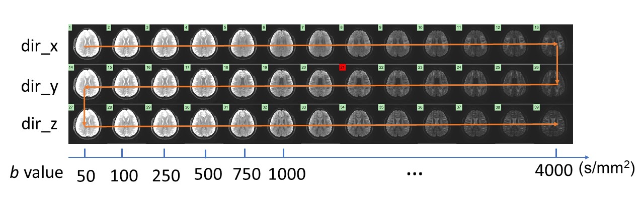
Figure 1: A set of multi-b-value DWI dataset from a representative slice showing the high degree of data redundancy among the images with different b-value and different diffusion directions.
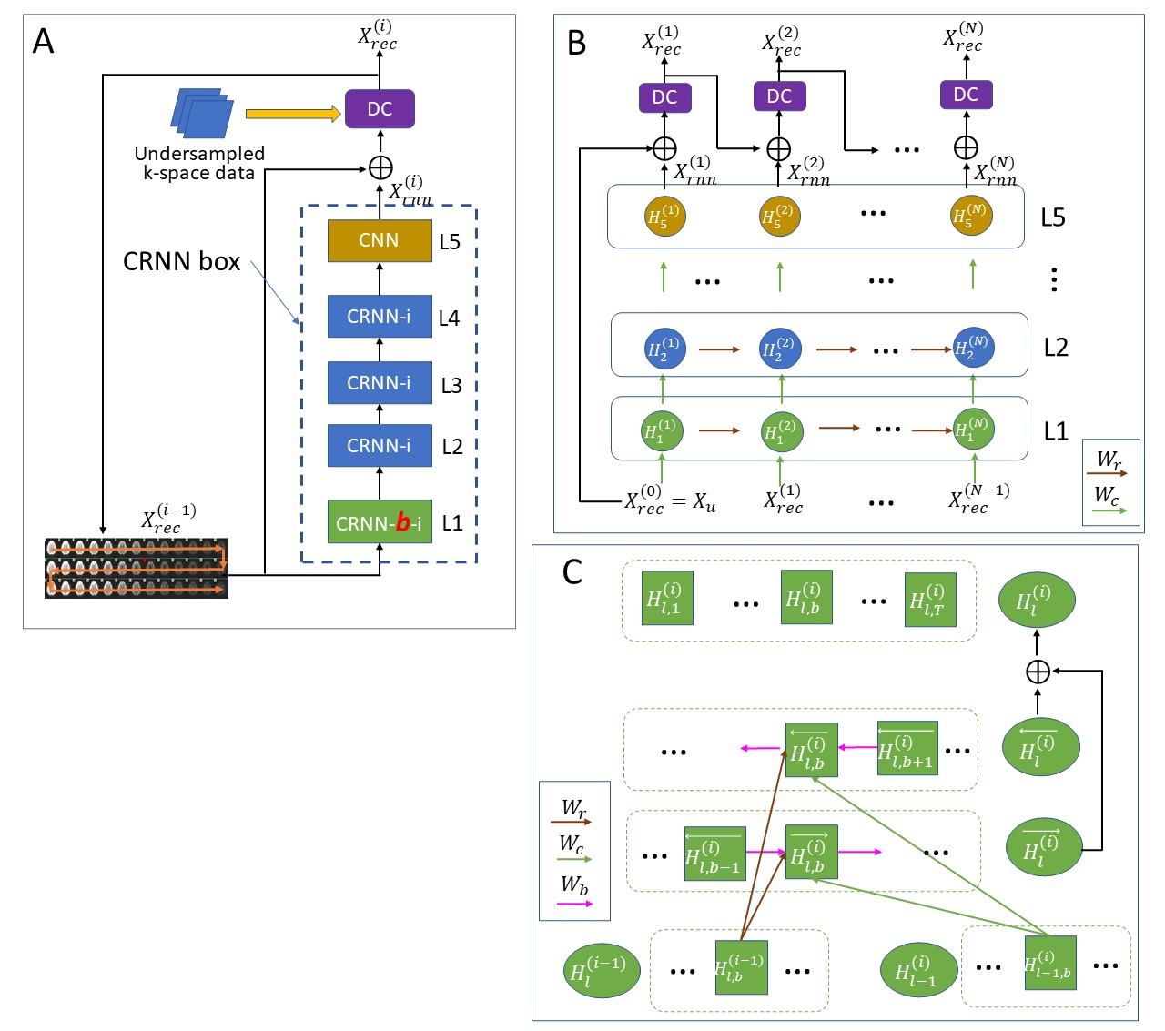
Figure 2: The structure of CRNN-DWI used in this study. (A): The detailed structure of the proposed network for each layer; (B): The unfolded structure of the proposed network for each iteration; and (C): The detailed structure of CRNN-b-i layer. The green arrow (Wc), brown arrow (Wr), and pink arrow (Wb) represent the filters of input-to-hidden convolutions, hidden-to-hidden recurrent convolutions evolving over iterations, and the b-value series, respectively.
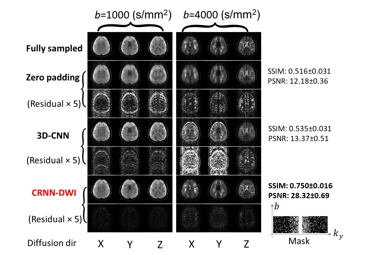
Figure 3: Representative images from the experiments with four-fold undersampling. The reconstructed images using CRNN-DWI outperformed 3D-CNN and were the closest to the ground truth for a broad range of b-values.
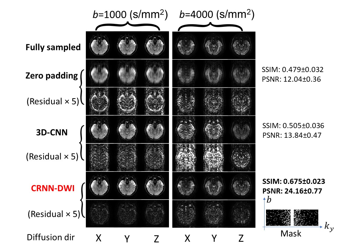
Figure 4: Representative images from the experiment with six-fold undersampling. The quality of the reconstructed images using CRNN-DWI is not as good as that with four-fold undersampling, yet still considerably out-performed 3D-CNN and zero-padding.
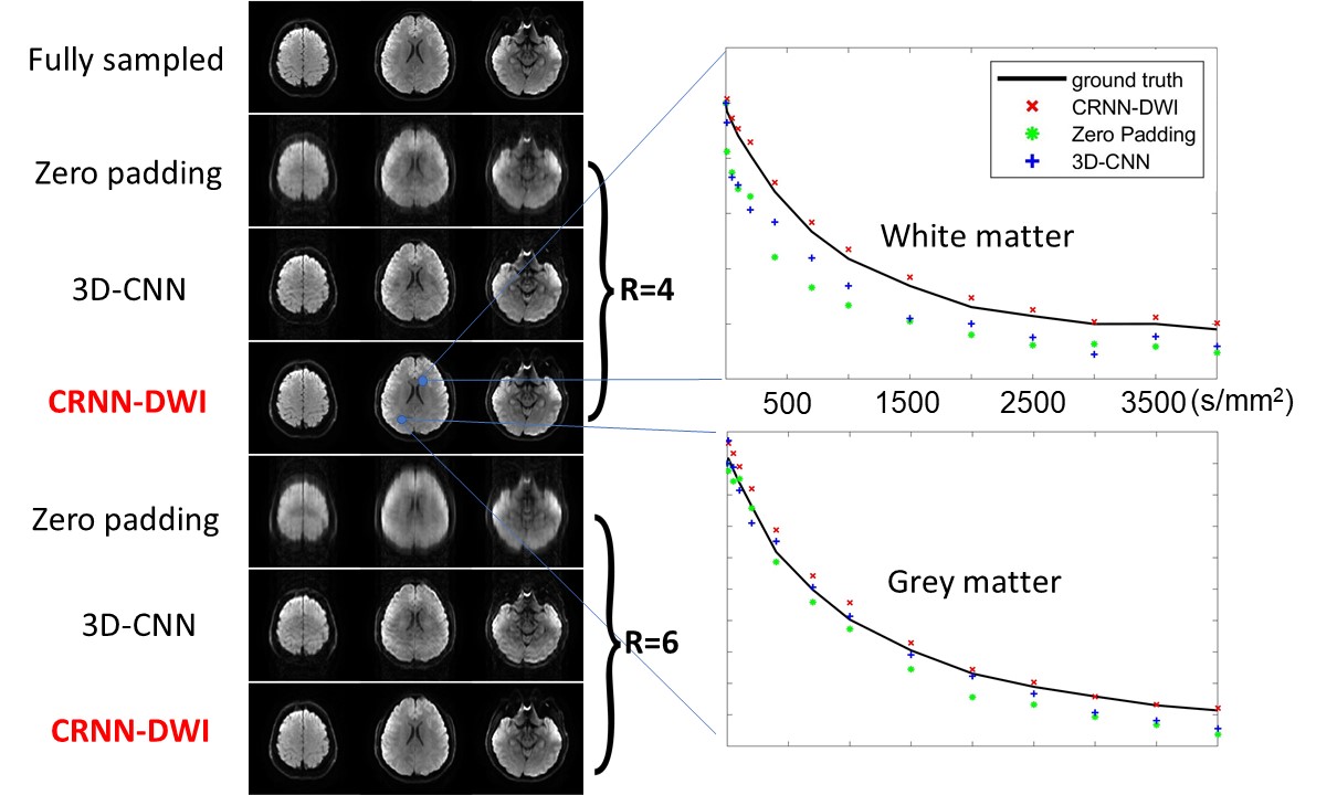
Figure 5: Representative trace-weighted images at b = 1000 s/mm2 (left) using different reconstruction methods and the corresponding signal decay curves (right) from two randomly selected ROIs (white matter and gray matter as indicated by the blue areas). The trace-weighted images reconstructed using CRNN-DWI showed excellent image quality even with a six-fold undersampling. The signal decay curves from CRNN-DWI agreed well with the curves using fully sampling images, whereas the curve from zero-padding and 3D-CNN exhibited substantial deviations.