Introduction

Most MR-exams intrinsically feature loud acoustic noise as the imaging gradients need to be switched fast and at high amplitude to ensure short acquisition times. Together with claustrophobia these loud sounds are the main sources of patient anxiety during MR-exams, which might lead to a degradation of the image quality (1,2). Previously, we have presented a silent gradient axis that aims to lower sound levels by providing extra soundless spatial encoding and allow the other imaging gradients to be switched slower, which reduces the sound level without loss of imaging time(3). In this work, we present the field characteristics and first images for a silent gradient designed for a clinical 3 tesla MR-system.

Methods

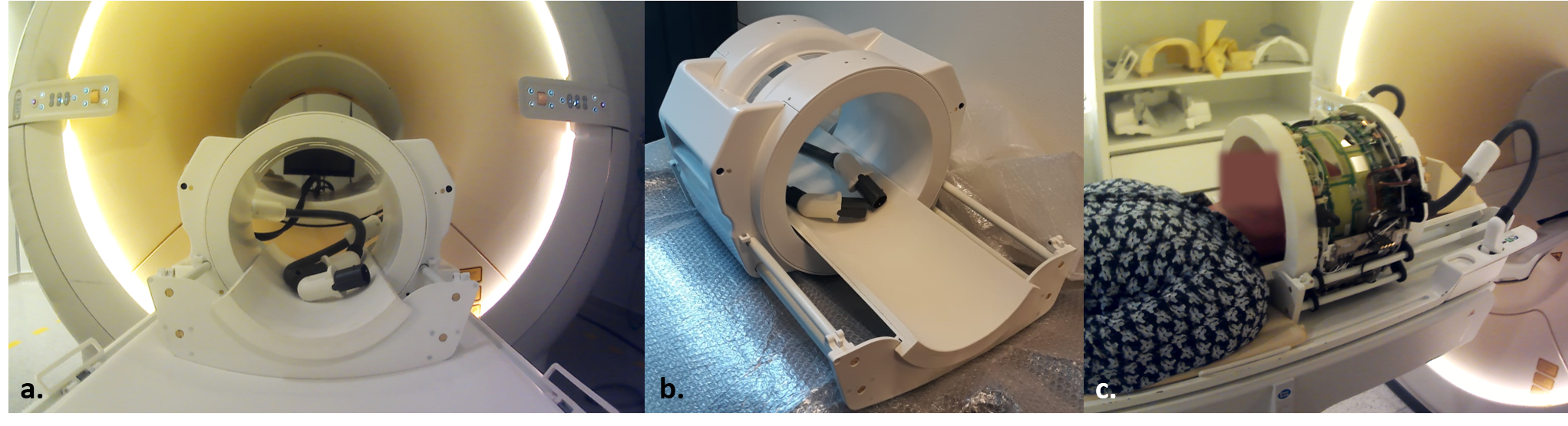
Gradient design
An open and lightweight design was targeted for the silent gradient (Futura composites, Heerhugowaard & Tesla DC, Zaltbommel). The silent gradient coil consisted of 32 windings distributed in two groups (16 windings per group), which were spaced 25 cm apart and produced a z-gradient field. By grouping the windings like this, the amount of epoxy needed to pot the gradient coil was minimized resulting in a weight of 21 kg of the whole coil, which facilitates easy installation comparable to a standard head coil. The gradient coil was made resonant at 23.5 kHz using two capacitors and combined with a modified gradient amplifier (NG500, Prodrive Technologies, Son) to maximize the silent encoding (4). Furthermore, a 32-channel receive coil array was integrated into the coil with the receive elements distributed over 4 rows extending in the feet-head direction to facilitate parallel imaging along the direction of the silent gradient. This receive array consisted of two attached PCB’s containing all coils which were decoupled based on a predetermined overlap. Figure 1 shows the final coil design.
Characterization
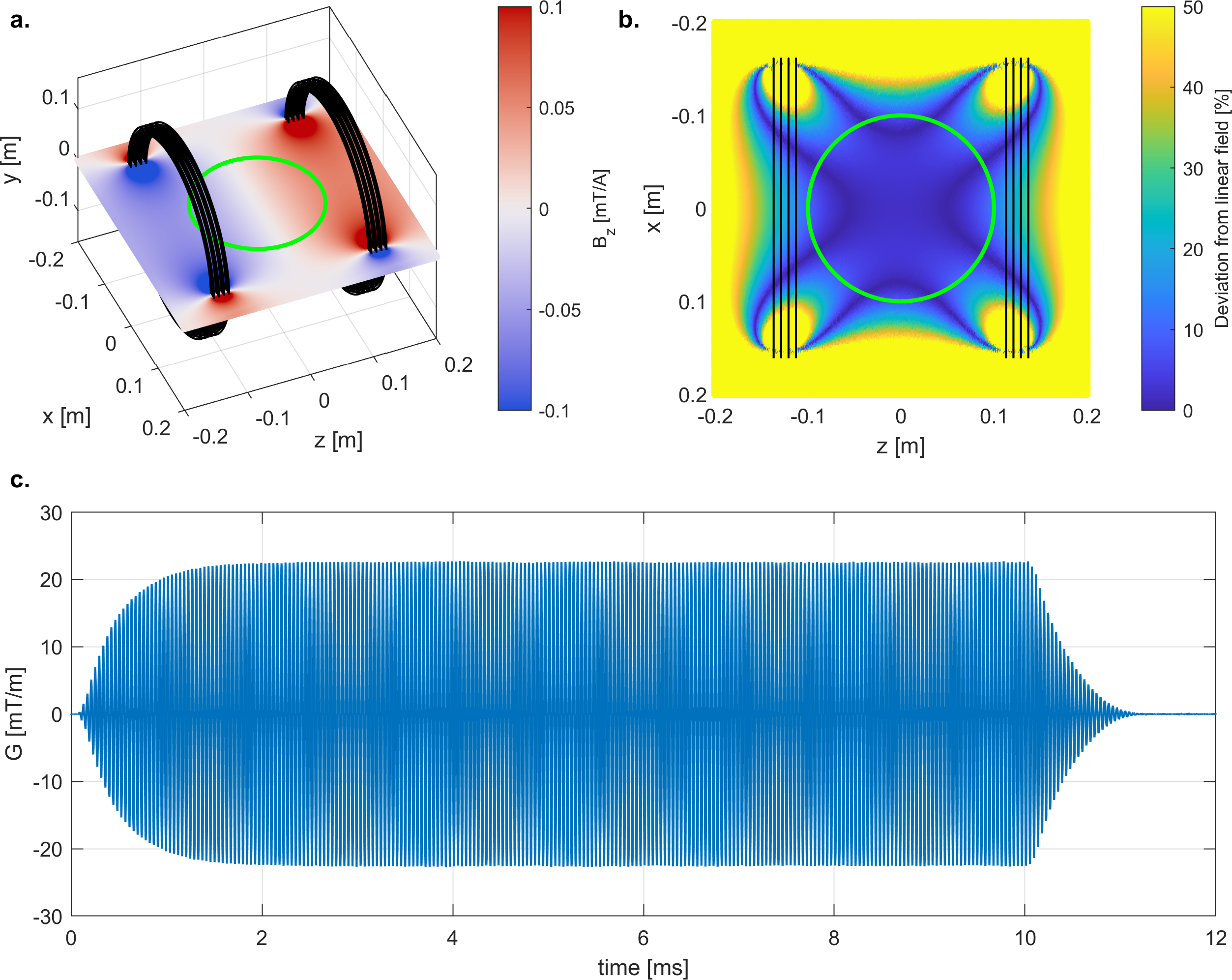
The gradient field distribution was calculated using the Biot-Savart law and was used to determine gradient efficiency and field linearity. The exact resonance frequency and spatiotemporal gradient field behavior were measured using a dynamic field camera (Skope Magnetic Resonance Technologies AG, Switzerland). During these measurements the gradient coil was positioned in a 7T MR-system (Philips, The Netherlands).
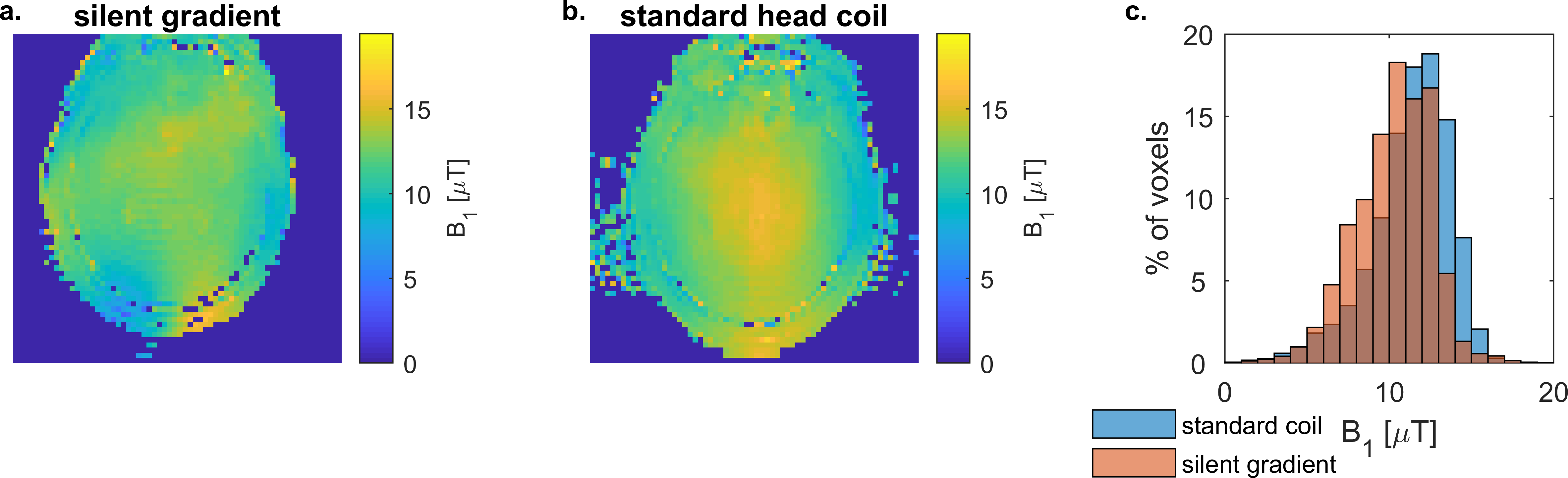
To investigate transparency of the setup to the transmit field of the 3T RF body-coil, B1-mapping was performed with the same subject, once with the setup and once with the standard Philips head coil.
Images
For imaging experiments, the RF coil array with the embedded silent gradient was positioned in a 3T MR-system (Ingenia CX, Philips, Best). A phantom consisting of a water-filled bottle was imaged to investigate the imaging performance along the linear region of the gradient. Here, a modified 2D gradient-echo sequence that plays out the silent gradient during readout was used with the following imaging parameters: coronal slice orientation, in-plane resolution = 2 x 2 mm², FOV = 256 x 512 (RL x FH) mm², slice-thickness = 4 mm, TE = 5.6 ms, TR = 60 ms, and flip angle = 16°. Additionally, a similar sequence was used to image a volunteer with the following imaging parameters: coronal slice orientation, in-plane resolution = 1 x 1 mm², FOV = 256 x 256 (RL x FH) mm², slice-thickness = 6 mm, TE = 21 ms, TR = 60 ms, and flip angle = 21°. All images were acquired with the silent gradient operating at 22.5 mT/m. Reconstruction was performed off-line in MATLAB using the field camera data and a non-uniform Fourier transform.

Results and Discussion

Figure 2a shows the field distribution of the silent gradient. Here, the gradient efficiency was determined to be 0.56 mT/m/A. Figure 2b shows the deviation from a perfectly linear gradient field for the silent gradient, which shows that the gradient field has less than 10% deviation from linearity in a 20 cm DSV. The field measurements in figure 2C shows the gradient field oscillating at 23.5 kHz and at an amplitude of 22.5 mT/m. Additionally, the silent gradient needs about 1.5 ms to reach a steady state and ~1 ms to return back to zero.

The B1-maps (Fig 3ab) shows similar performance with both setups in the MR-system suggesting that the interaction with the gradient coil is limited. On average the B­1 measured with the silent gradient system was ~10% lower. However, the B1-field homogeneity was not affected as the distribution of B1-values (Figure 3c) was similar for both setups (σ_{B1-silent­ gradient} = 2.3 µT vs σ_{B1-standard coil} = 2.4 µT).

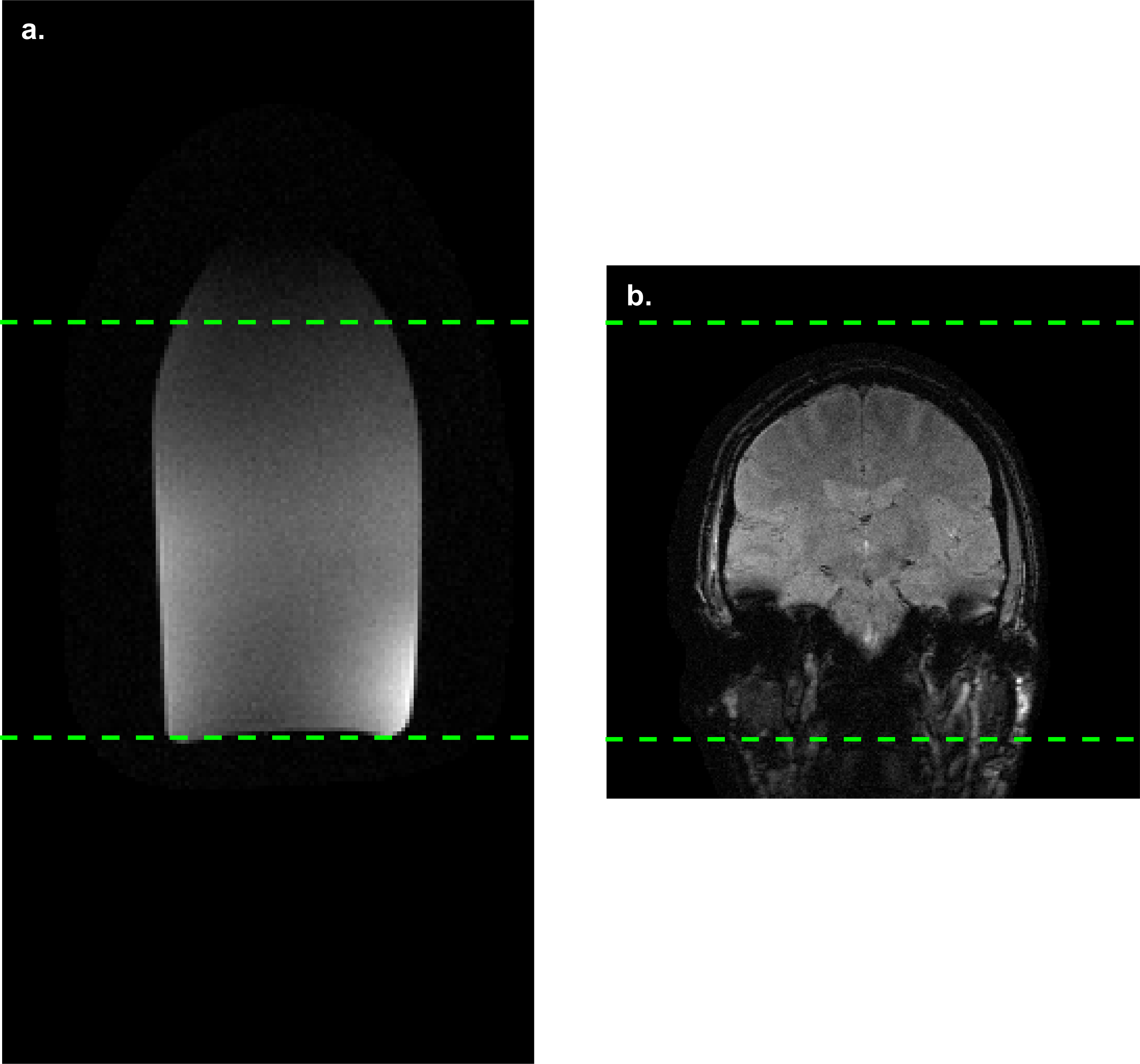
Figure 4a shows that no significant distortion is observed over the 20 cm linear region. However, some signal loss was seen outside this region, which might be recovered by incorporating the field non-linearity in the reconstruction. In Figure 4b, the in-vivo image shows that the whole-brain fits in the 20 cm linear region.

Earlier work on silent gradient axes was performed at 7 tesla, where a 26 dB reduction in sound level was achieved for a T1-weighted anatomical scan (5). Translating the concept of the silent gradient axis to 3 tesla is expected to yield similar or lower sound levels as the Lorentz forces at 3 tesla are intrinsically lower.

Conclusion

We have presented a silent gradient designed for 3 Tesla MR-system, which can enable quiet and fast brain imaging.

Acknowledgements

No acknowledgement found.