Introduction

Accurate gradient fields are mandatory for spatial encoding in MRI, and any deviation from predefined gradient waveforms results in image artifacts. One source of perturbation is gradient heating due to ohmic losses in the coils caused by gradient currents. The gradient heating increases the coil resistance, which alters the current flowing through the coils if there is no feedback in the system. Feedback control based on measuring the output current can eliminate this perturbation^1,2; however, it necessitates expensive current sensors. Feedforward control^3,4 based on the linear time-invariant (LTI) model is susceptible to thermal variations because of the underlying assumption of time invariance. As a result, model parameters deviate from the expected values. This work aims to model the thermal variation of gradient coil winding to predict and update feedforward control parameters by solving the thermal equation numerically. The proposed system is free from expensive current sensors, and therefore it reduces the cost of the gradient array technology.

Methods

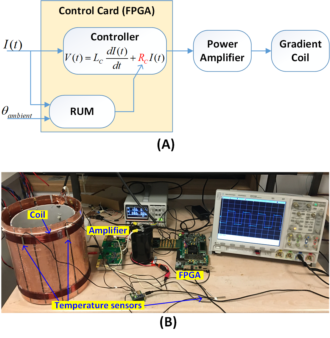
The LTI model used in feedforward controllers is:
$$V(t)={L_C}\frac{{dI(t)}}{{dt}}+{R_C}I(t)\quad (1)$$
However, time-invariance can be violated due to temperature variation. High currents flowing through the gradient coil cause a temperature rise in various parts of the gradient system, mainly in the coil winding. This increase affects the resistance of the gradient coil (R_C), which alters the output current. The well-known linear relationship between temperature and resistance is as follow:
$${R_C}(t)={R_C}({t_0})\left({1+\alpha\left({\theta(t)-\theta ({t_0})}\right)}\right)\quad (2)$$
Here α is the temperature coefficient of copper wire. R_C(t₀) and θ(t₀) are the initial values of the coil’s resistance and temperature, respectively.
To improve the controller performance, the R_C parameter in Eq.1 must be updated based on coil temperature. The thermal differential equation determines the temperature of a current-carrying conductor.
$$\frac{{d\theta }}{{dt}}={k_1}{R_C}(t){I^2}(t)-{k_2}\left({\theta(t)-{\theta_{ambient}}}\right)\quad (3)$$
The solution of this equation is an inverse exponential with a time constant of $$$\tau=\frac{1}{{{k_2}-k_1\alpha{R_C}({t_0}){I^2}}}$$$. We measure the temperature variation of coil winding while applying a constant voltage to the coil to determine k₁ and k₂. The system block diagram and measurement setup are depicted in Fig.1. The resistance updating module (RUM) calculates the temperature and the coil’s resistance based on an arbitrary input current waveform and the ambient temperature, and updates the RC parameter in the feedforward controller. To demonstrate the efficiency of the proposed method, we drive the coil with a 5-minute continuous trapezoidal waveform (non-stop EPI readout, 30A peak current), with and without RUM, and measure the coil current at the start and end of the sequence. To distinguish temperature-dependent effects from the nonlinear imperfections, we also employ a nonlinear model4 that compensates for the droop originating from system nonlinearities.

Results

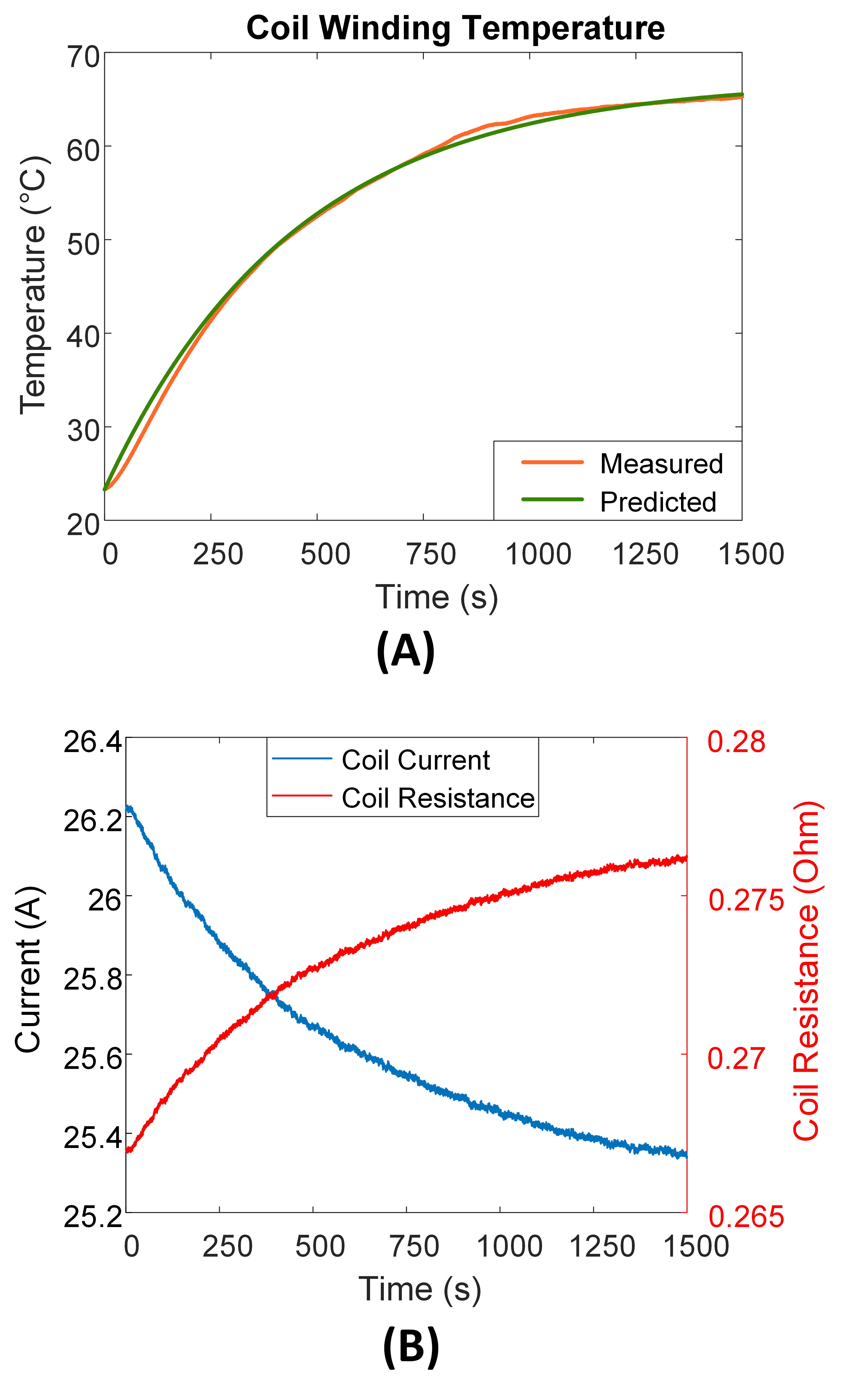
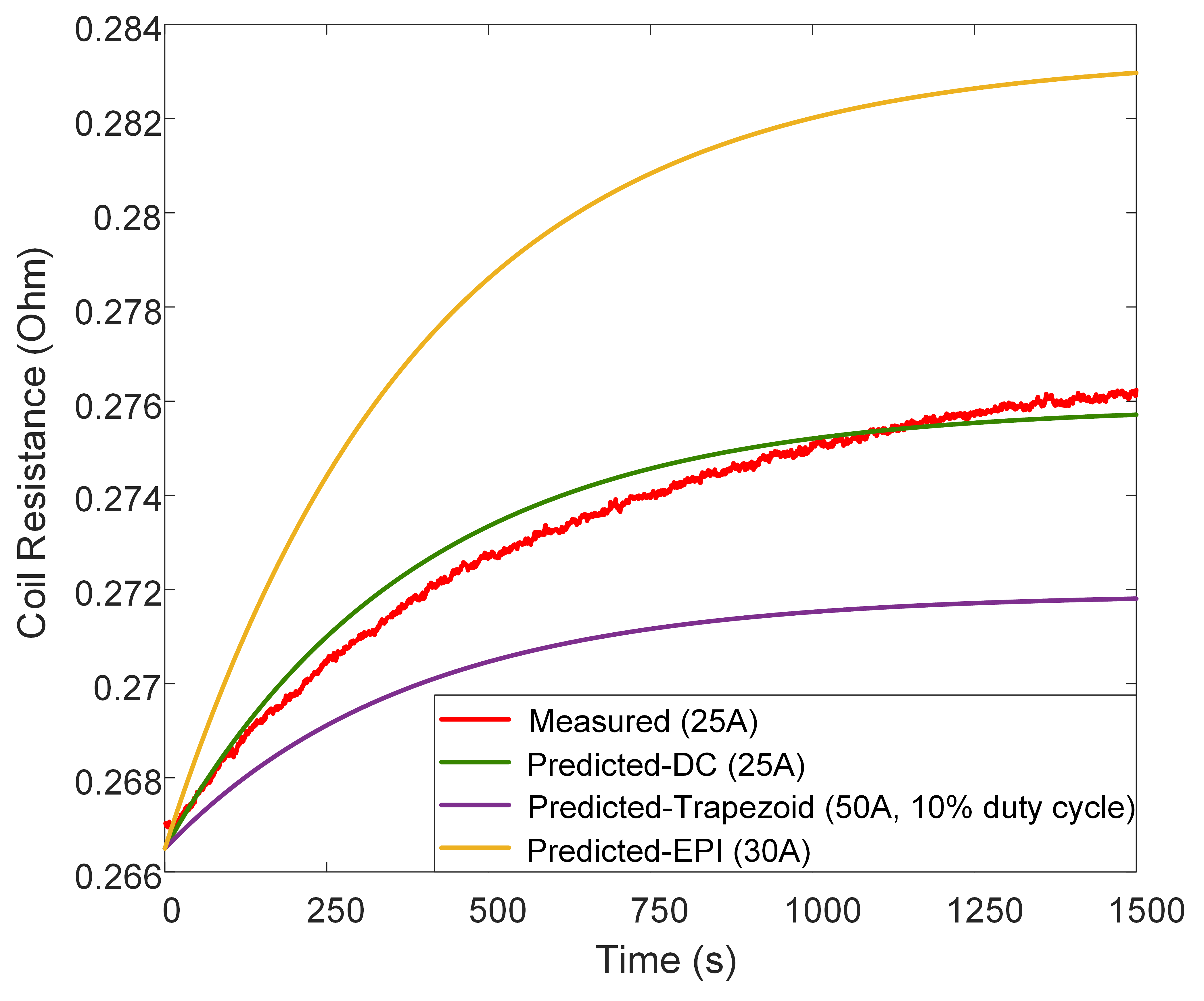
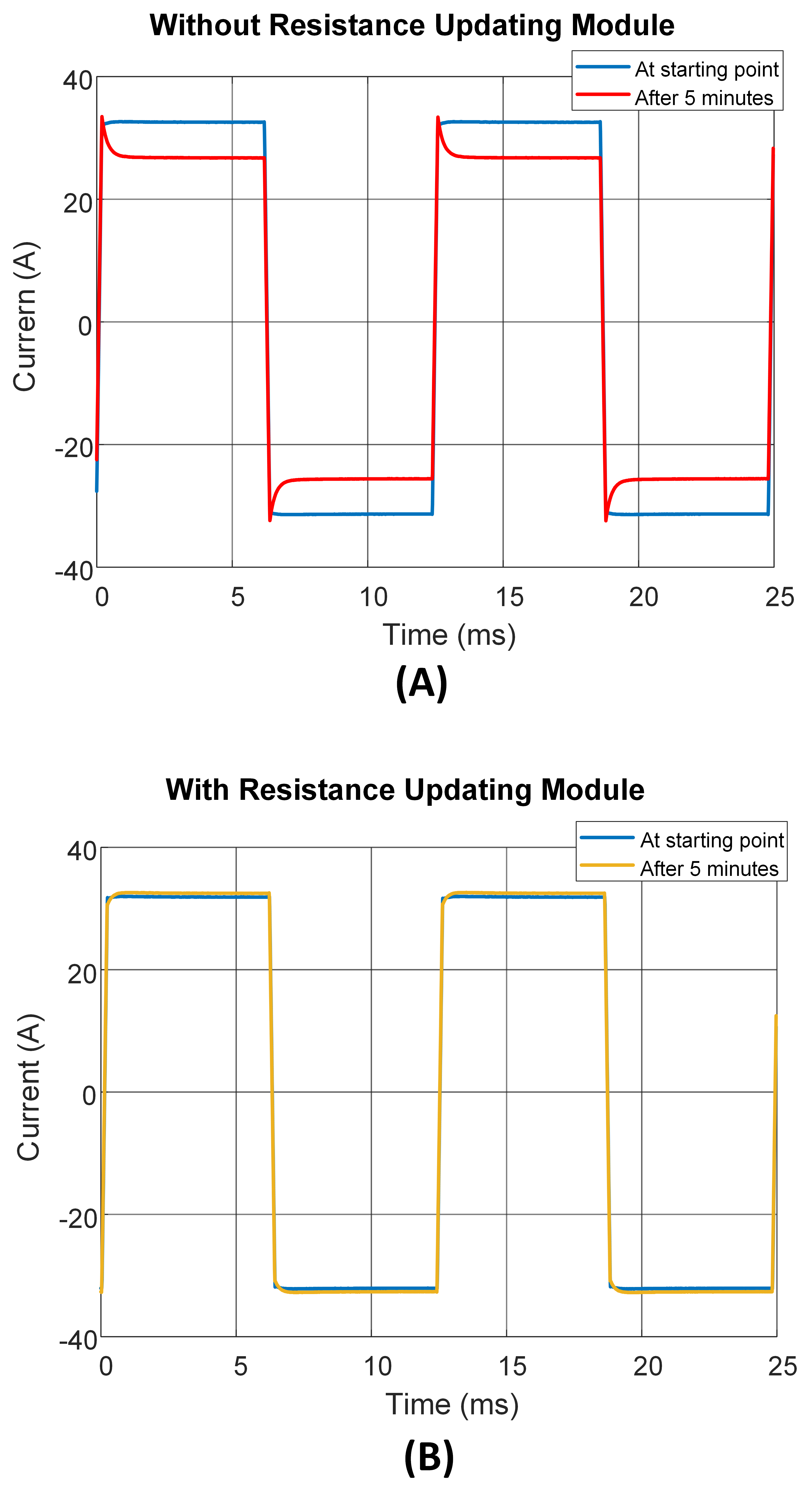
Fig.2A depicts a good match between the measured and predicted temperatures of the coil winding, indicating the thermal equation’s accuracy. The ambient temperature was 23.3 °C, and by applying a 25A DC current for 25 minutes, the temperature will reach its steady-state (66 °C). Fig.2B shows the coil resistance and the current flowing through the coil versus time for the LTI model without the updating feature. As a result of the gradient coil heating, the coil resistance increases, and the current decreases from its starting value. Our measurements show a 3.8% decrease in current, but it is higher for higher amplitude currents. Fig.3 shows a good agreement between the measured (red) and predicted (green) coil resistances. However, the residual errors could be caused by the heating of the gradient power amplifier, as we only considered coil winding resistance in the thermal equation calculation. The predicted coil resistances when applying a trapezoid current with 50A peak amplitude (10% duty cycle) and EPI readout waveform with 30A peak current are shown in Fig.3 (purple and yellow, respectively). Fig.4 demonstrates the coil current measurements at the onset and after 5 minutes while applying the continuous trapezoidal waveform, with and without RUM. The coil’s current begins with the desired waveform; however, with fixed model parameters, its amplitude gradually decreases due to gradient heating (Fig.4A). The reduction is greater than our predicted value because the power amplifier heating causes an additional reduction in the current. By activating the updating block, the feedforward controller will be able to provide the desired current at the output, as shown in Fig.4B.

Discussion

In this study, we update the time-variant parameter of the feedforward controller by predicting the thermal behavior of the gradient coil based on the input current and ambient temperature. Our measurements confirmed that the LTI model, which is prone to time-varying parameters, cannot provide accurate waveforms as variations in the coil resistance alter the output current. The proposed method updates the LTI model parameters to achieve the desired waveform. Here, we only considered the gradient coil winding and not the gradient power amplifier in the thermal prediction process, which results in some errors in our prediction. However, the thermal behavior of the amplifier can be taken into account, resulting in an additional thermal equation. Due to the lack of a water cooling system, measurements were conducted with currents less than 30A. We expect the accurate functionality of the proposed method in the presence of a cooling system, which will only change the rate of heat transfer and thus the system time constant.

Acknowledgements

No acknowledgement found.