Introduction

Certain MRI applications, including spiral and ultrashort echo-time (UTE) imaging, require obtaining an accurate gradient trajectory that often deviates from the prescribed waveform. The deviation can be attributed to factors such as gradient delay, eddy currents, and gradient amplifier imperfection encompassing nonlinear components coming mainly from PID (proportional–integral–derivative) feedback. Existing trajectory correction techniques include gradient field measurement, gradient system response (GSR) calibration, and delay correction, among others [1-5]. Gradient field measurement can obtain accurate trajectory but is impractical in the clinical scan where gradient waveform changes with user-specified parameters thus would require re-measurement. Other correction techniques mostly rely on the assumption of linearity, assuming the MRI gradient system can be modeled by an impulse response function. However, as will be shown, the above assumption is not valid and will cause artifacts.


In this study, a versatile, practical, and effective gradient trajectory correction technique that considers gradient system nonlinearity is proposed and validated on phantoms and human subjects. It incorporates deep neural network (DNN) to predict actual gradient waveforms from prescribed waveforms as input. After system setup, additional calibration is not needed during scanning. To our knowledge, this is the first time DNN has been employed to solve MRI gradient system problems.

Methods

Gradient waveform measurement: Following exciting a thin slice perpendicular to the gradient axis, the to-be-measured gradient was played with simultaneous signal receiving. Four different slice positions were used, and polarities of the gradients were varied to remove confounding factors, similar to previously published [6].

GSR calibration: A series of triangle waveforms with different amplitudes were prescribed and measured. Sample waveforms (Figure 1) were shown at a similar scale to emphasize nonlinearity features that are not scalable. GSR was calculated following the previous approach [5].

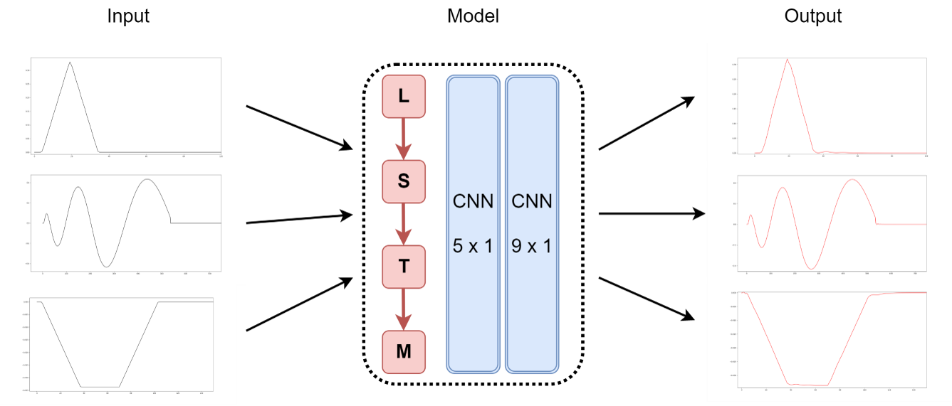
DNN architecture and training: The task could be viewed as a signal reconstruction problem where the model attempts to a generate measured waveform, with the prescribed waveform as the input. The most popular deep learning architecture for image or signal reconstruction is U-Net and its variants which consist of an encoder and a decoder [7-9]. However, gradient waveforms are predefined functions that contain more global features (overall shape) than local features (texture), and therefore using a convolutional operation would not be effective. Instead, a long short-term memory (LSTM) architecture is proposed (Figure 2). The feedback connection in LSTM allows the network to remember the entire sequence of the dataset, which helps the model memorize the waveform shapes as well as their amplitude. After LSTM, two convolution layers are added to reconstruct waveforms from extracted features.

The LSTM contained one hidden layer with 100 dimensions, and the two convolution layers had kernel sizes of 5x1 and 9x1, respectively. Mean squared error loss function and Adam optimization were used. The initial learning rate was 0.01 and reduced by half when the validation loss was not improved after 20 consecutive epochs. The model was trained with 500 epochs, and the weight that yielded the lowest validation loss was saved. Duration and amplitude of triangle, spiral and trapezoid gradients, whose shapes are commonly used in MRI scans, were varied to generate different waveforms. A total of 1517 waveforms were recruited for training. Data augmentation was employed by inverting gradient polarity and time-shifting waveforms.

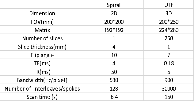
Study experiment: All data were acquired on a clinical 3T scanner (uMR790, United Imaging Healthcare, Shanghai, China). 2D spiral imaging and 3D UTE imaging with koosh ball trajectory were performed on phantoms and human brains (Table 1). For comparison, reconstruction was conducted using the following waveforms: the measured actual waveforms (as gold standard), waveforms predicted using GSR, waveforms predicted using the proposed DNN, and the prescribed waveforms. Care was taken not to use waveforms already in the DNN’s training dataset for imaging. Reconstruction involved regridding with Kaiser-Bessel kernel, density compensation, and sum-of-squares coil combination.

Results

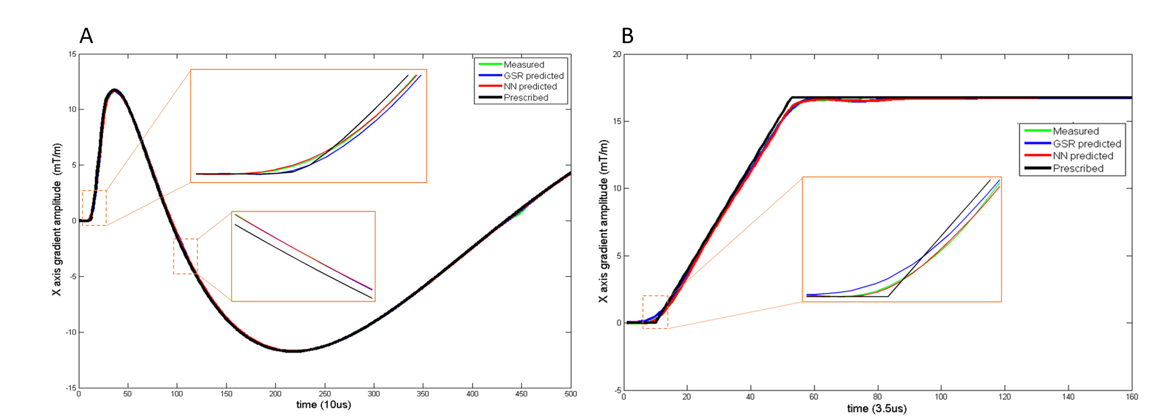
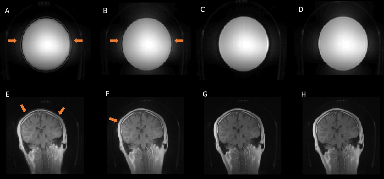
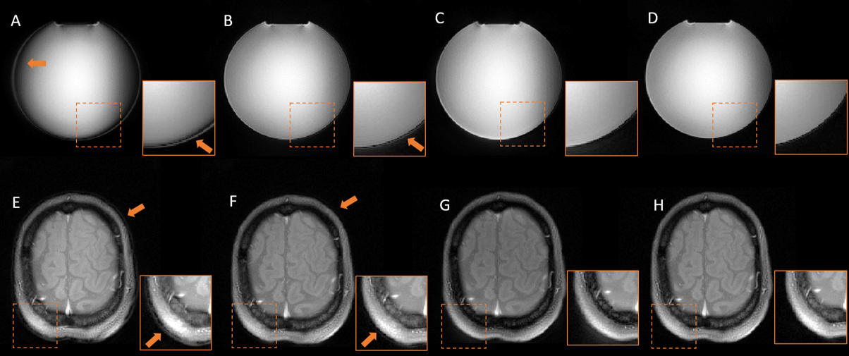
Typical spiral and UTE gradient waveforms from the various methods are illustrated in Figure 3. Compared to GSR, DNN waveforms have better agreement with the gold standard, particularly at low-amplitude which correspond to the region around k-space center that contributes heavily to image contrast. Phantom and volunteer images (Figures 4 and 5) reconstructed with DNN waveforms are free of artifacts present in those with GSR and have similar image quality to the gold standard.

Conclusion and Discussion

The feasibility of using DNN for gradient waveform prediction was demonstrated and showed superior image quality than the conventional GSR method by incorporating the nonlinearity response. Despite that only predicting gradient waveform is demonstrated in this study, applying the same approach to predicting B0 eddy current should be straightforward. In response to the large amount of data needed for DNN training, future work will be directed towards accelerating model training by transfer learning between 1) scanners of the same model, 2) scanners of different models but same field strength, and 3) scanners of different field strengths.

Acknowledgements

No acknowledgement found.