0584
MRI-based measurement of the transfer function of elongated metallic implants without transceive phase approximation.
Michael Eijbersen1,2, Bart Steensma1,2, Cornelis A.T. van den Berg1,2, and Alexander J.E. Raaijmakers1,2,3
1Radiotherapy, UMC Utrecht, Utrecht, Netherlands, 2Computational Imaging Group, UMC Utrecht, Utrecht, Netherlands, 3Biomedical Engineering, Eindhoven University of Technology, Eindhoven, Netherlands
1Radiotherapy, UMC Utrecht, Utrecht, Netherlands, 2Computational Imaging Group, UMC Utrecht, Utrecht, Netherlands, 3Biomedical Engineering, Eindhoven University of Technology, Eindhoven, Netherlands
Synopsis
A new computational method is presented for determining a transfer function of implants using a MRI only paradigm. By relaxing the transciever phase approximation better results are obtained for longer implants, however an optimization for both B1+ and B1- based on magnitude only maps is required.
Introduction
The transfer function (TF) is an important characteristic of elongated implant structures. It relates the incident electric field along the implant to the electric field enhancement at the tip of the implant. The assessment of the transfer function is part of the RF safety assessment for MRI-safe labelling as prescribed in the ISO standard [1]. The transfer function is conventionally measured using a bench setup. However, Tokaya et al introduced an alternative method where the MRI system is being used to measure the transfer function of elongated implant structures in an ASTM phantom from the artefacts that the induced RF currents generate [2]. The method, however, assumes negligible z-components of the B1-field (transceiver phase approximation), which is only valid for relatively short implant structures. In this work, we introduce an improved computational method to asses the transfer function of an implant, without this assumption making the method applicable for implant wires/leads as long as the field of view of the scanner. Using simulated data generated by a model in Sim4Life we show that this computational method is more accurate than previous work.Materials and Methods
The MRI-based TF measurement techniques makes use of the concept of the transfer matrix (TM) which relates incident electric fields along the implant to induced current on the implant:$$I=ME_{inc}$$.
A parameterized version of the TM can be determined if incident Ez-field and induced current are known. From Maxwell’s equations we may derive the relation between measured B1- fields and the Incident Ez-fields.
$$ E_z=\frac{1}{\mu_0\sigma+i\omega\mu_r\mu_0\epsilon_r\epsilon_0}\left(-i\frac{\partial B^{1+}}{\partial x}-\frac{\partial B^{1+}}{\partial y}+i\frac{\partial B^{1-}}{\partial x}-\frac{\partial B^{1-}}{\partial y}\right)$$
The transceive phase approximation assumes $$$\frac{\partial Bz}{dz}=0$$$ in which case the following relation holds:
$$\frac{\partial B_1^{+}}{\partial x}+i\frac{\partial B_1^{+}}{\partial y}=-\frac{\partial B_1^{-}}{\partial x}+i\frac{\partial B_1^{-}}{\partial y}$$
This allows the incident electric field to be determined by only B1+. If the assumption is not valid, both field components need to be determined which, for a homogeneous phantom, can be obtained from the proton density scaling factor in the multi-flip angle B1-measurement method [2,3]. Induced current is determined by fitting the B1+ and B1- fields to a EM field model where the background field is modeled as a superposition of spherical harmonics while the scattered field is modeled through Jefimenko’s generalization of the Biot-Savart law:
$$B_{1,bg}^{\pm}=\sum_{n,l,m} j_l(kr)Y^l_m(\theta,\phi)$$ $$B_{1,sc}^\pm(\vec{r})\exp(i\omega t)=\frac{4\pi}{\mu_0}\int_{\text{wire}}I^\pm(\vec{r}')\exp\left(t-\frac{|\vec{r}'-\vec{r}|}{c_m}\right)\left(\frac{1}{|\vec{r}'-\vec{r}|^3}+\frac{i\omega}{c_m|\vec{r}'-\vec{r}|^2}\right)dr'\times (\vec{r}'-\vec{r})$$
The combined scattered and background field (d) in the data may be written as a matrix vector product:
$$\vec{d}=A\vec{x}+J\vec{y}$$
Here the matrix A and J contain discretized versions of the background and scattered field terms respectively. Since only magnitudes of the data points are available in experiments, the problem is reformulated in a Magnitude Squared Least Squares (MSLS) setting. This allows for working with inner products which are linear and allows us to rewrite the problem in terms of z, which is the concatenation of x and y with their real and imaginary part splitted. In this formulation we may derive equations for the cost function, gradient and hessian in order to use a Trust Region Newton algorithm to find an acceptable local minimum. A schematic representation of the derivation is provided in figure 2.
The proposed method was tested using simulated |B1+| and |B1-| field distributions of a realistic birdcage body coil in the conventional ASTM phantom (ϵr = 78.0 and σ = 0.34 S/m) which contains a 42 cm insulated copper wire (figure 1). Resulting Ez and Iind vectors were used to determine the TM of which the first column is the TF.
Results and Discussion
Figure 3 shows the simulated B1+ and B1- distributions along with the corresponding reconstructed EM field models. Clearly, the model captures the behavior of background and scattered field very well. The reconstructed Ez and Iind values along the wire are indicated in figure 4 along with their simulated ground-truth counterparts. Computation of Ez using only B1+ based on the transceiver phase approximation clearly shows unacceptable deviations from the ground truth in this case. Data shows that both magnitude and phase reveal some minor deviations, which do not severely affect the TF accuracy. The resulting normalized TM and TF are presented in figure 5 along with the ground truth simulated counterparts. These results show that the proposed method is capable of calculating the transfer function from MRI-accessible data, even for longer implants where the transceive phase approximation is no longer valid.Conclusion
A MRI-based measurement method for TF determination without restrictive assumptions was presented. For this purpose, a calculation pipeline was developed to acquire incident electric fields from B1+ and B1- distributions. A EM-model was setup to parameterize the background-scattered field combination. Application on simulated field distributions shows that the method is capable of determining the transfer function from MRI-accessible data.Acknowledgements
No acknowledgement found.References
- Implants ISA. Iso/ts 10974:2012(en). Assessment of the safety of magnetic resonance imaging for patients with an active implantable medical device. 2012
- Tokaya, Janot P., et al. MRI‐based transfer function determination through the transfer matrix by jointly fitting the incident and scattered field. Magnetic resonance in medicine, 2020, 83.3: 1081-1095.
- van den Bosch, Michiel R., et al. New method to monitor RF safety in MRI‐guided interventions based on RF induced image artefacts. Medical physics, 2010, 37.2: 814-821.
Figures
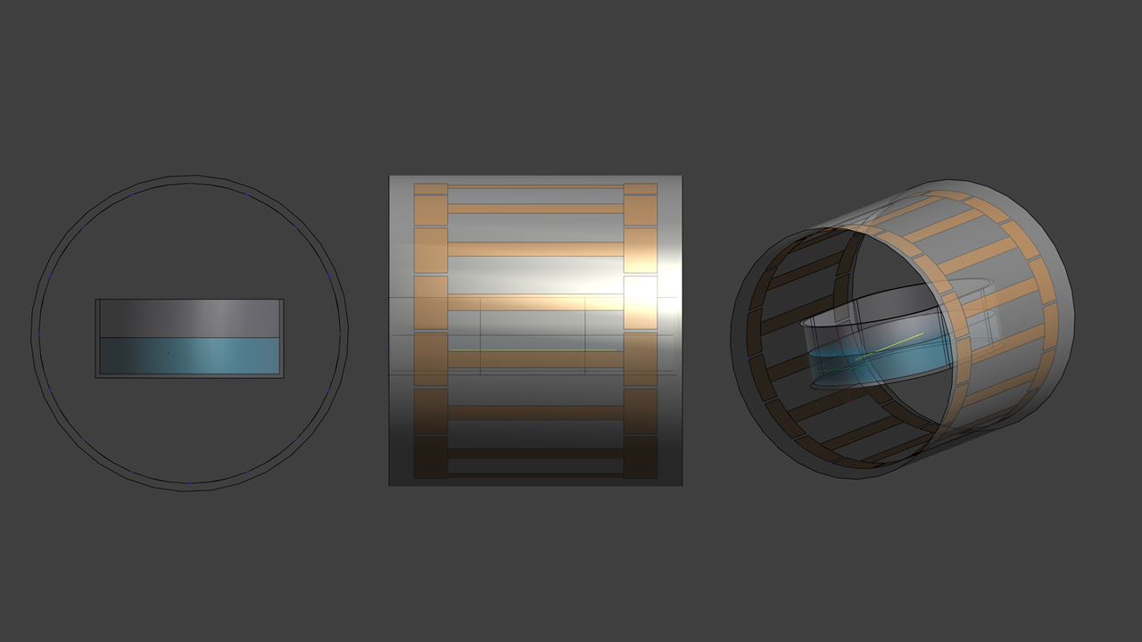
Figure 1: The Sim4Life model from three perspectives.
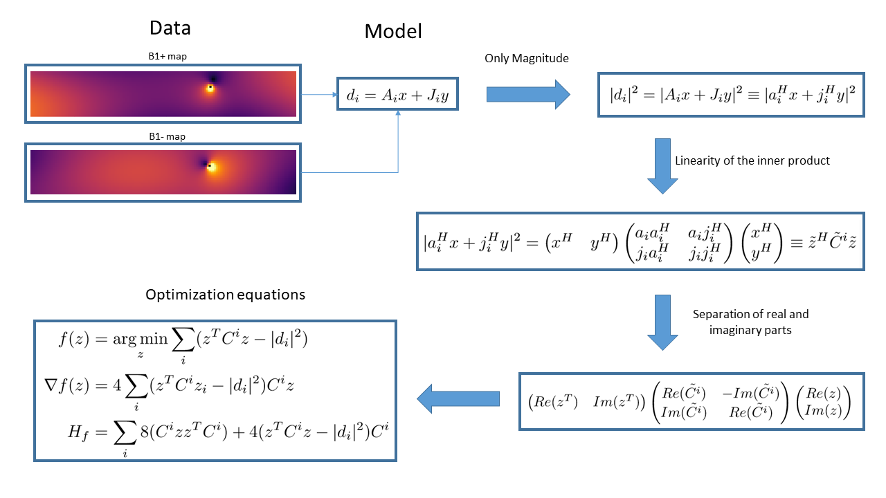
Figure 2: The Mathematics behind the MSLS formulation of the problem. By taking the magnitude squared it is possible to use the linearity of the inner product and separation of real and imaginary parts to derive the optimization equations. Note that $$$A_i \equiv a_i^H$$$ and $$$A_i \equiv a_i^H$$$ and $$$J_i \equiv j_i^H$$$ to make vectors lower case and non-hermitean vectors columns.
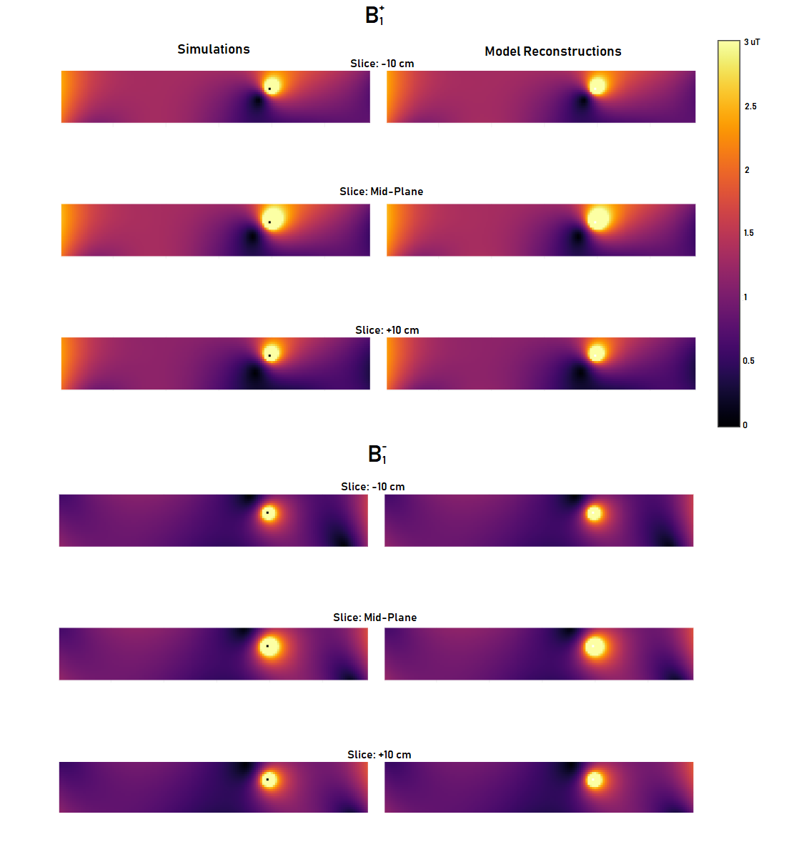
Figure 3: The results of the optimization compared with the simulations. The images show excellent agreement for both B1+ and B1-.
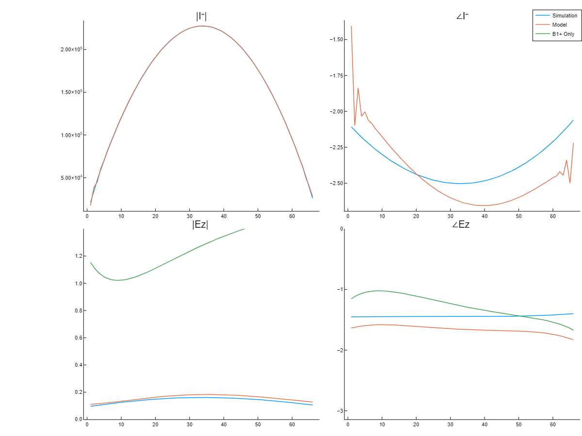
Figure 4: Comparison between the simulated induced current and incident electric fields. Note that the calculated incident electric field based on the transciever phase approximation yields an unacceptable estimate.
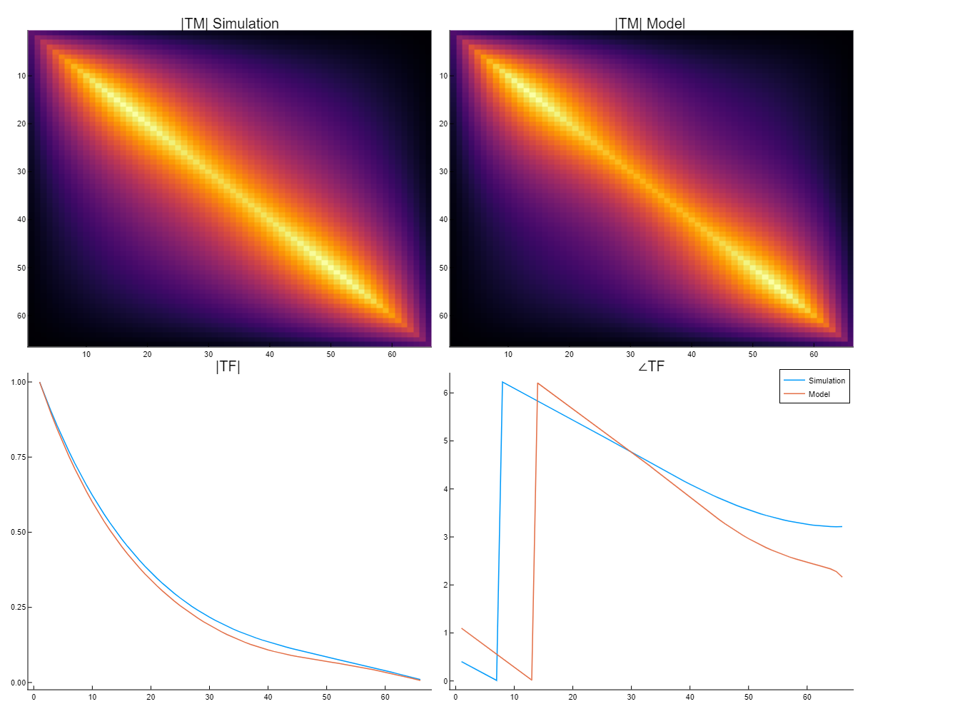
Figure 5: A comparison of the Transfer Matrix and Transfer functions between the simulation and the model reconstructions. The transfer function shows good agreement.
DOI: https://doi.org/10.58530/2022/0584