0579
Influence of electric field and axon geometry on peripheral nerve stimulation chronaxie1Harvard Graduate Program in Biophysics, Harvard University, Cambridge, MA, United States, 2Harvard-MIT Division of Health Sciences and Technology, MIT, Cambridge, MA, United States, 3Computer Assisted Clinical Medicine, Medical Faculty Mannheim, Heidelberg University, Heidelberg, Germany, 4A. A. Martinos Center for Biomedical Imaging, Department of Radiology, Massachusetts General Hospital, Charlestown, MA, United States, 5Harvard Medical School, Boston, MA, United States
Synopsis
We calculate the impact of peripheral nerve geometry (bend angle, radius of curvature, and axon diameter) and electric field characteristics (hot-spot amplitude and extent) on the chronaxie of nerve stimulation to better understand the variability in experimental chronaxie values seen with MRI gradient coils.
Introduction
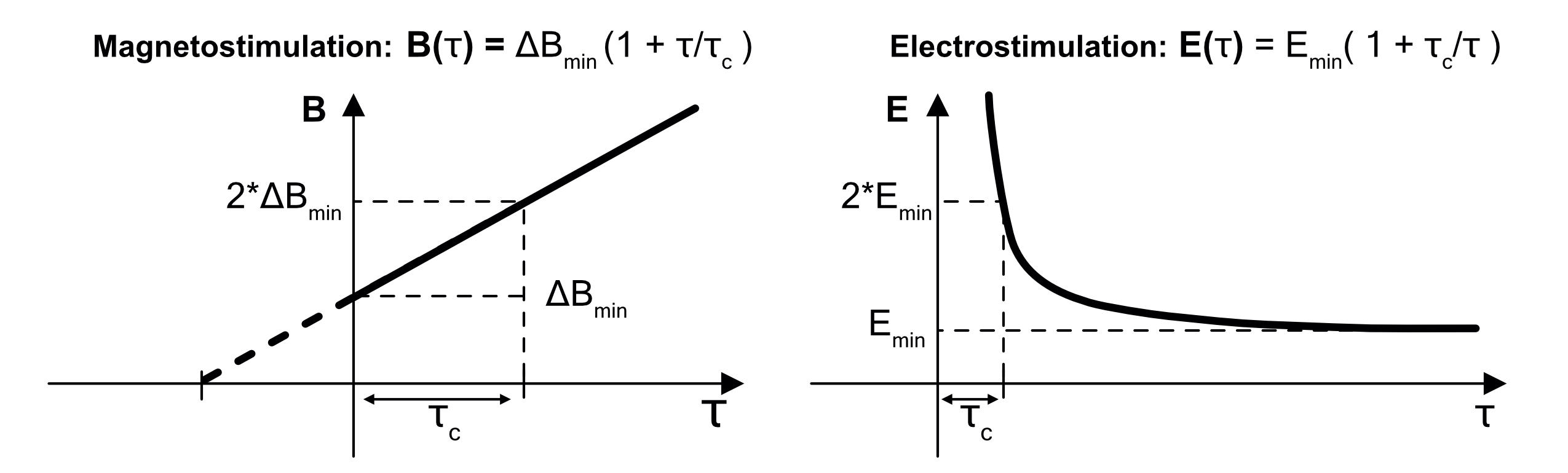
The Peripheral Nerve Stimulation (PNS) strength-duration threshold curve is typically characterized by the experimentally-determined minimum stimulating gradient amplitude as a function of risetime for a periodic waveform, B(τ) = ΔBmin (1 + τ / τc ) (Eq. 1), where the chronaxie, τc, is defined as the pulse duration (2x risetime) of the waveform whose threshold is twice ΔBmin (Fig 1.)1-4.Significant variation in experimental chronaxie values have been reported for MRI gradients with values ranging from 138-810μs for body gradients1,5-13 and 285-1100μs for head gradients6,14-15. Additionally, electrostimulation experiments show that chronaxie varies with the spatial pattern of the electric stimulus seen by a nerve fiber3,4,16,17, type of nerve18, and physiologic parameters19-22. The IEC 60601-2-3323 guidelines include setting PNS safety limits for whole-body gradients based on an assumed chronaxie of 360μs. Using a predetermined chronaxie value for a gradient whose experimental chronaxie deviates from that value may lead to incorrect predictions by the PNS safety monitor.
The variability seen in experiments underscores the importance of better understanding how nerve geometry and field shape relate to chronaxie. Here we evaluate how different peripheral nerve geometries (bend angle, radius of curvature, and axon diameter) and E-field characteristics (hot-spot amplitude and extent) alter the expected chronaxie of PNS. The differing chronaxie values reported for different coils could then be interpreted in terms of the specifics of the individual location from which the threshold arises which can be expected to differ from coil to coil (especially between body and head gradients).
Methods
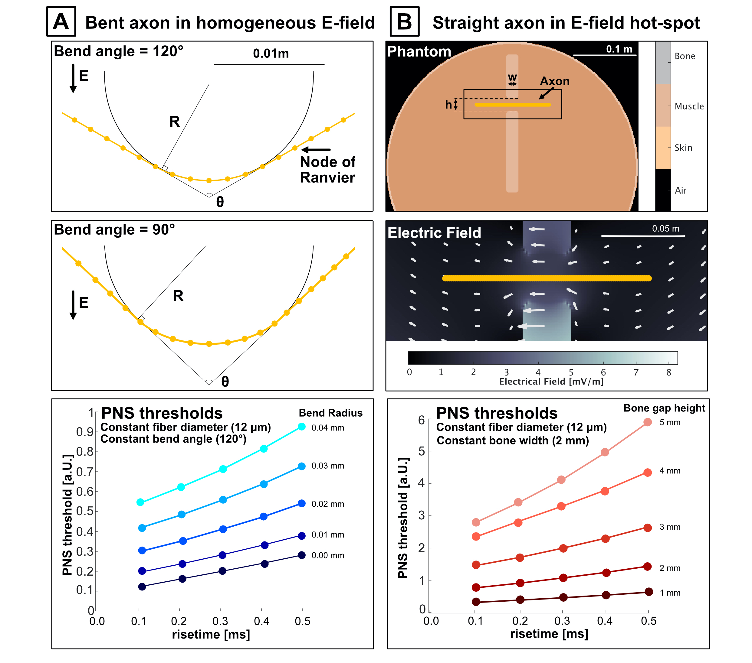
We use our previously published PNS model24-25 based on a coupled electromagnetic-neurodynamic modeling approach. For a given E-field pattern and nerve fiber geometry, we project the E-field onto the nerve and integrate the result to obtain electric potential changes along the nerve. We then predict the response of the nerve using the McIntyre-Richardson-Grill (MRG) double-cable model26. Results were obtained for trapezoidal waveforms (0.1–0.5ms risetime, 16 bipolar pulses, 0.5ms flat top).To isolate geometric impacts on chronaxie, we focus on two simplistic artificial cases and study how the parameters modulate chronaxie as well as the axonal driving function (DF), defined as the second spatial derivative of the electric potential along the nerve27. Figure 2A shows the case of a bent nerve in a homogeneous E-field consisting of straight segments intersecting with bend angle, θ, connected by a circular segment with bend radius, R. We study chronaxie as a function of θ and R. Figure 2B shows the case of a straight nerve segment embedded in a simplistic body-model mimicking E-field hot-spot formation from bottlenecking body structures. The configuration consists of a cylindrical object with skin, muscle, and low-conductivity bone; the nerve segment passes through a bone gap of varying width and height. Figure 2 also reports the PNS thresholds as a function of risetime for both cases. We obtain the nerve chronaxie by fitting Eq. 1 to the PNS thresholds.
Results
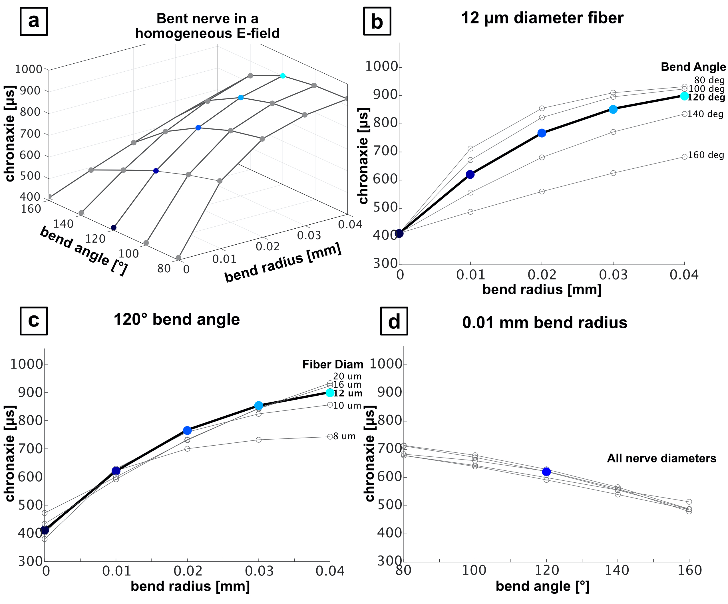
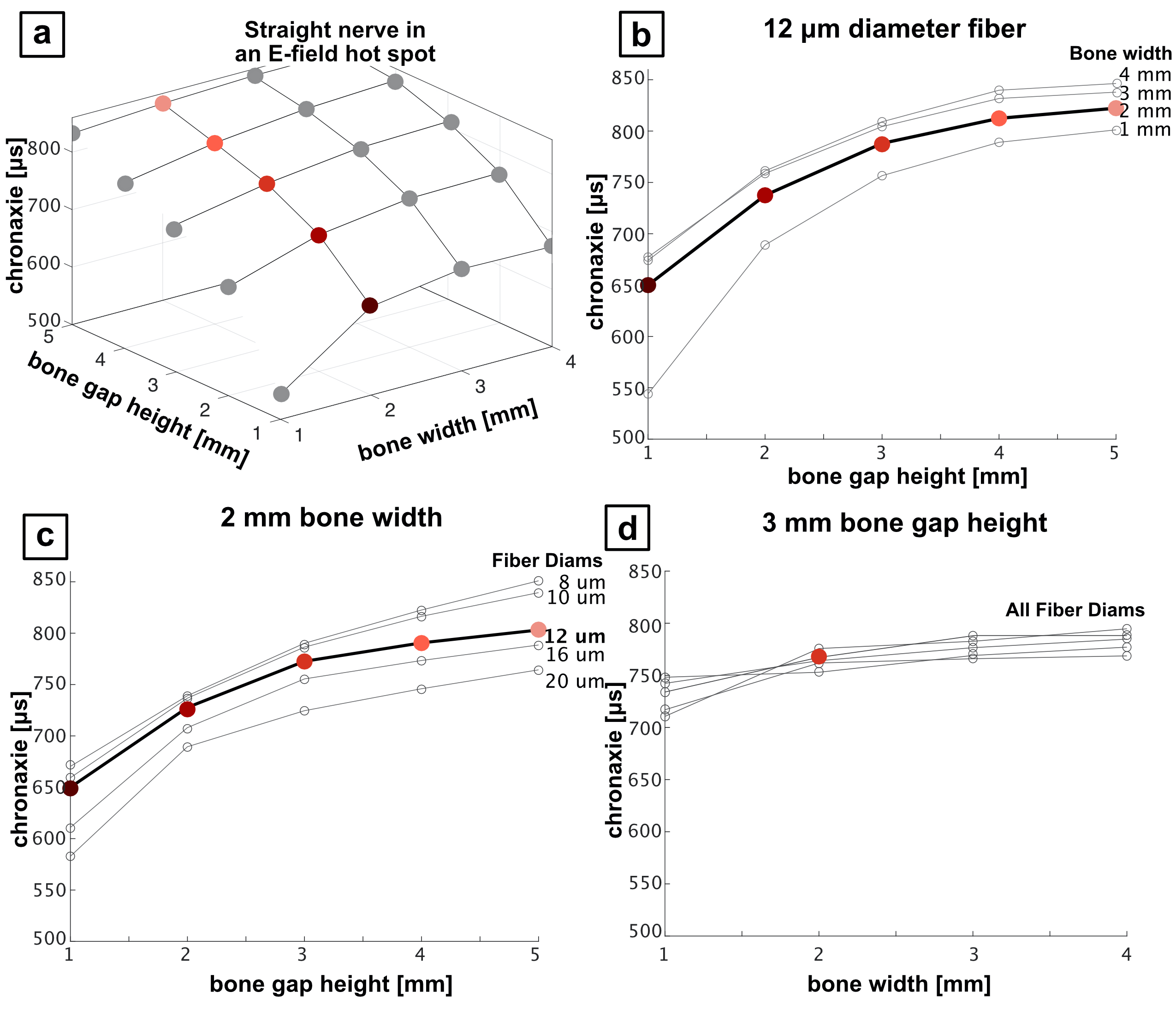
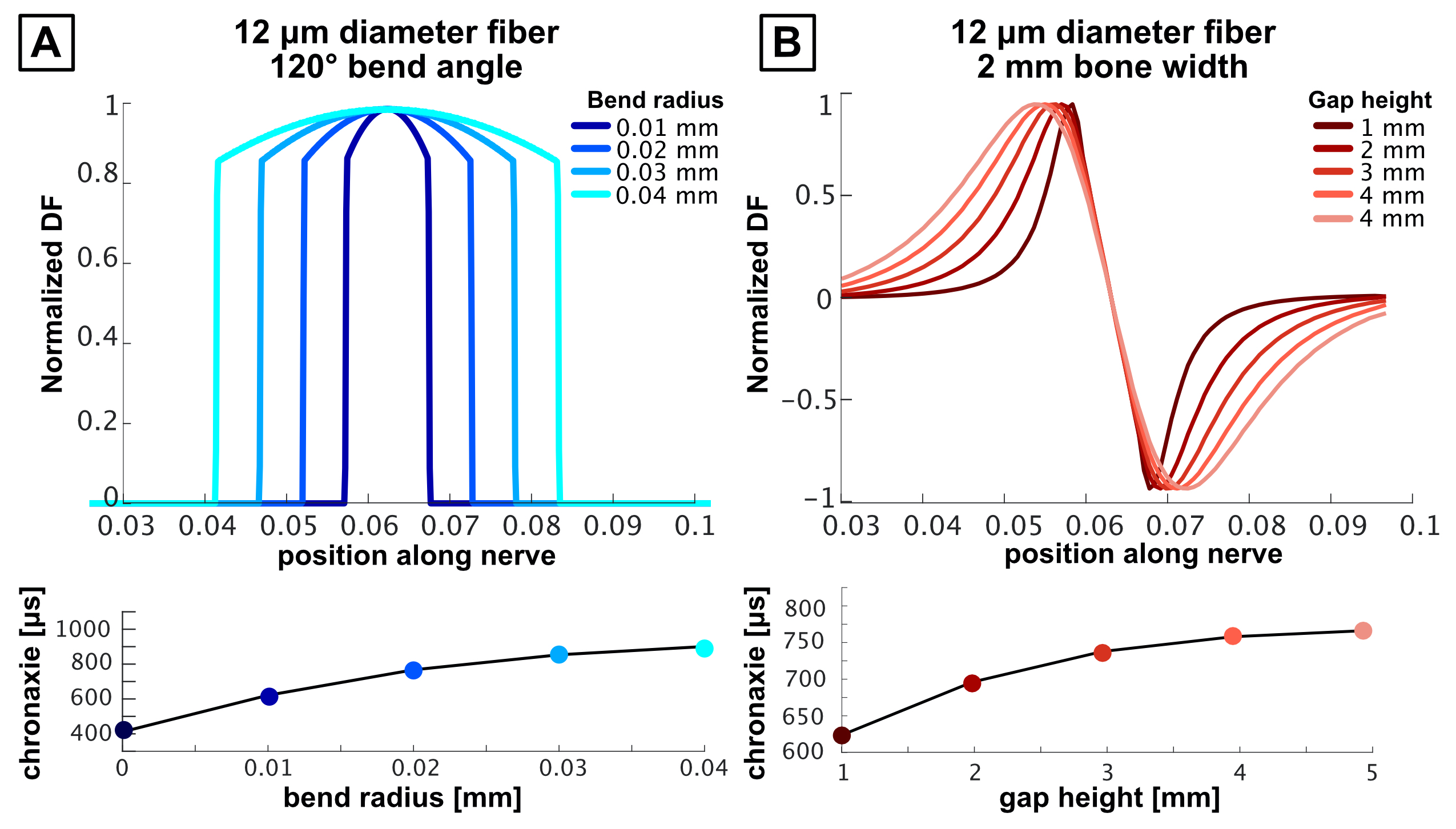
Figure 3 shows chronaxie results from the bent axon parameterization (Fig. 2A) as a function of θ and R for different axon diameters. Figure 3b shows constant bend angle slices from the surface plot in Fig. 3a. For all bend angles, the chronaxie asymptotes towards a maximum value with increasing bend radius. Fig. 3c shows the chronaxie as a function of bend radius for constant axon diameter. Larger axons have longer chronaxies in the limit of large bend radius. In Fig 3d, chronaxie values for a single bend radius are plotted as a function of bend angle for all axon diameters. For the case of a single bent axon in a homogeneous E-field, the range of parameters shown here result in chronaxies that range from 380 to 1050μs.Figure 4 shows chronaxie results from the straight axon parameterization (Fig. 2B) as a function of bone width and bone gap height for different axon diameters. The bone width determines the width of the stimulus seen by the axon whereas the bone gap height impacts the maximum amplitude of the E-field. For the case of a straight axon in a varying E-field hot-spot, chronaxie ranged from 545 to 850μs.
Figure 5 shows normalized DF to compare nodal activation between axons with different chronaxies. The magnitude of the DF provides information about the polarization of each node and is a proxy for PNS thresholds. We plot the normalize the axonal DF to isolate the impact of DF width on chronaxie. In both cases, broader DF corresponds to a longer chronaxie.
Discussion
In this work we show how the axon chronaxie is influenced by both the axon geometry and the local E-field shape with the width of the driving function indicating of the resulting chronaxie. A wider DF indicates a greater number of nodes are depolarized in response to the external stimulus leading to a lower potential drop between neighboring nodes. This results in slower dissipation of current along the axon making the PNS threshold less sensitive to changes in pulse duration (longer chronaxie). This supports the view that the chronaxie of a gradient coil is dictated by the topology of the most sensitive axon and the local field and could be expected to vary with coil-type and body position.Acknowledgements
NSF GRFP DGE1745303
NIH NIBIB grant R01EB028250
Funding from Siemens Healthineers
References
[1] Irnich W and Schmitt F. Magnetostimulation in MRI. Magn. Reson. Med., 33(5):619–623, 1995.
[2] Irnich W. The chronaxie time and its practical importance. Pacing Clin. Electrophysiol., 3(3):292–301, 1980.
[3] Irnich W. Electrostimulation by time-varying magnetic fields. MAGMA., 2:43-49, 1994.
[4] Recoskie BJ, Scholl TJ, and Chronik BA. The discrepancy between human peripheral nerve chronaxie times as measured using magnetic and electric field stimuli: the relevance to MRI gradient coil safety. Phys. Med. Biol., 54(19):5965, 2009.
[5] Chronik BA and Rutt BK. A comparison between human magnetostimulation thresholds in whole-body and head/neck gradient coils. Magn. Reson. Med., 46(2):386–394, 2001.
[6] Ham CLG, Engels, JML van de Wiel GT, and Machielsen A. Peripheral nerve stimulation during MRI: Effects of high gradient amplitudes and switching rates. J. Magn. Reson. Imaging, 7(5):933–937, 1997.
[7] Den Boer JA, Bourland JD, Nyenhuis JA, Ham CLG, Engels JML, Hebrank FX, Frese G, and Schaefer DJ. Comparison of the threshold for peripheral nerve stimulation during gradient switching in whole body MR systems. J. Magn. Reson. Imaging, 15(5):520–525, 2002.
[8] Reilly JP. Peripheral nerve stimulation by induced electric currents: exposure to time-varying magnetic fields. Med Biol Eng Comput 1989: 27:101–110.
[9] Setsompop K, Kimmlingen R, Eberlein E, et al. Pushing the limits of in vivo diffusion MRI for the human connectome project. Neuroimage. 2013;80:220-233.
[10] Bourland J, Nyenhuis J, Schaefer D. Physiologic effects of intense MR imaging gradient fields. Neuroimaging Clin N Am. 1999;9:363-377.
[11] Nyenhuis J, Bourland J, Foster K, Graber G, Kildishev A, Schaefer D. Magnetic stimulation in humans by MRI pulsed gradient fields. In: Proceedings of the IEEE Engineering in Medicine and Biology 21st Annual Conference and the 1999 Annual Fall Meeting of the Biomedical Engineering Society, Atlanta, Georgia, 1999. p 1074.
[12] Irnich W, Hebrank FX. Stimulation threshold comparison of time- varying magnetic pulses with different waveforms. J Magn Reson Imaging. 2009;29:229-236.
[13] Glover PM. Interaction of MRI field gradients with the human body. Phys Med Biol. 2009;54:99.
[14] Roemer PB, Wade T, Alejski A, McKenzie CA, Rutt BK. Electric field calculation and peripheral nerve stimulation prediction for head and body gradient coils. Magn Reson Med. 2021;86:2301-2315.
[15] Zhang B, Yen YF, Chronik BA, McKinnon GC, Schaefer DJ, and Rutt BK. Peripheral nerve stimulation properties of head and body gradient coils of various sizes. Magn. Reson. Med., 50(1):50–58, 2003.
[16] Saritas EU, Goodwill PW, Zhang GZ, and Conolly SM. Magnetostimulation limits in magnetic particle imaging. IEEE Transactions on Medical Imaging, 32(9):1600–16107, Sept 2013.
[17] Dhar SK, Heston KJ, Madrak LJ, Shah BK, Deger FT, and Greenberg RM. Strength duration curve for left ventricular epicardial stimulation in patients undergoing cardiac resynchronization therapy. PACE, 32:1146–1151, 2009.
[18] Mogyoros I, Kiernan MC, and Burke D. Strength-duration properties of human peripheral nerve. Brain, 119(2):439–447, 04 1996.
[19] Geddes LA. Accuracy limitations of chronaxie values. IEEE Transactions on Biomedical Engineering, 51(1):176–181, 2004.
[20] Geddes LA and Bourland JD. Tissue stimulation: Theoretical considerations and practical applications. Med. Biol. Eng. Comput., 23:131–137, 1985.
[21] Brismar T. Electrical properties of isolated demyelinated rat nerve fibers. Acta physiologica scandinavica, 113(2):161–166, 1981.
[22] Bostock H. The strength-duration relationship for excitation of myelinated nerve: computed dependence on membrane parameters. The Journal of Physiology, 341(1):59–74, 1983.
[23] Commission International Electrotechnical, International standard IEC 60601 medical electrical equipment. Part 2-33: Particular requirements for the basic safety and essential performance of magnetic resonance equipment for medical diagnosis. 2010, International Electrotechnical Commission (IEC).
[24] Davids et al. "Prediction of peripheral nerve stimulation thresholds of MRI gradient coils using coupled electromagnetic and neurodynamic simulations." Magnetic resonance in medicine 81.1 (2019): 686-701.
[25] Davids M, Guérin B, Malzacher M, Schad LR, Wald LL. Predicting magnetostimulation thresholds in the peripheral nervous system using realistic body models. Sci Rep. 2017;7:5316.
[26] McIntyre et al., “Modeling the excitability of mammalian nerve fibers: Influence of afterpotentials on the recovery cycle”. J Neurophysiol. 87(2), 2002.
[27] Peterson et al., Predicting myelinated axon activation using spatial characteristics of the extracellular field, J Neural Eng, 2011.
Figures