0561
Sequence optimisation mitigating undersampling errors in Magnetic Resonance Fingerprinting1Department of Imaging Physics, Delft University of Technology, Delft, Netherlands, 2Department of Numerical Analysis, Delft University of Technology, Delft, Netherlands, 3Department of Radiology and Nuclear Medicine, Erasmus MC, Rotterdam, Netherlands
Synopsis
In MR Fingerprinting acquisitions, the choice of flip angle sequence has a strong effect on the accuracy of the estimated parameter maps. Undersampling artefacts in time-series images are a dominant source of error for standard MRF estimations. We propose to use an undersampling-error model leveraging on perturbation theory, to optimise flip angle patterns taking into account the k-space readout, a realistic ground truth and signal phase. In vivo scans show strong visible reduction in error. Root-mean-square errors in $$$T_1$$$ and $$$T_2$$$ were reduced with at least 6.4%-points and 9%-points respectively, compared to a Cramér-Rao bound optimised and a conventional pattern.
Introduction
Magnetic Resonance Fingerprinting (MRF) comprises the undersampled imaging of transient spin states while varying flip angles are applied1. Undersampled acquisitions with zero-filled reconstruction result in large artefacts in the time-series images. For short acquisitions, undersampling artefacts are a dominant source of error in the reconstructed $$$T_1$$$ and $$$T_2$$$-maps.Sequence optimisation for MRF can be a powerful tool to increase accuracy of parameter maps or to reduce scan time2. Most previous attempts to optimise experiment design, modelled noise and undersampling artefacts as an independent and identically distributed stochastic process with mean zero, effectively neglecting that undersampling artefacts cause spatial correlations between voxels3,4. Here we use the previously introduced undersampling model by Stolk and Sbrizzi5 to optimise the MRF flip angle sequence for increased robustness to undersampling errors. The effectiveness of the optimised sequences is verified using simulations and in vivo scans.
Theory
In this work we aim to estimate the tissue parameters $$$\boldsymbol{\theta} = (T_1, T_2, \text{Re}(\rho\exp(i\omega)), \text{Im}(\rho\exp(i\omega)))^{T}$$$ with $$$\rho$$$ being the real valued proton density and $$$\omega$$$ the signal phase. The matching procedure is effectively a voxel-wise least-square estimate based on the undersampled time-frame images $$$\boldsymbol{I}(\vec{x})$$$:$$\boldsymbol{\theta}^{*}(\vec{x}) =\operatorname*{argmin}_{\tilde{\boldsymbol{\theta}}}||\boldsymbol{I}(\vec{x}) - \boldsymbol{M}(\tilde{\boldsymbol{\theta}}(\vec{x}))||^{2},$$ where $$$\boldsymbol{M}(\tilde{\boldsymbol{\theta}}(\vec{x}))$$$ is the modelled transverse magnetisation for tissue parameters $$$\tilde{\boldsymbol{\theta}}$$$. To obtain a closed form expression for the reconstructed quantitative maps $$$\boldsymbol{\theta}^{*}$$$, the stationary point of the objective function above can be expanded using perturbation theory:\begin{align}\boldsymbol{\theta}^{*}(\vec{x}) &= \boldsymbol{\theta}_0 + \boldsymbol{\theta}_1^{*}(\vec{x}),\\\boldsymbol{\theta}(\vec{x}) &= \boldsymbol{\theta}_0 + \boldsymbol{\theta}_1(\vec{x}),\end{align}with $$$\boldsymbol{\theta}$$$ denoting the true tissue parameters. Here $$$\boldsymbol{\theta}_0$$$ is the spatial average of the tissue parameters, while $$$\boldsymbol{\theta}_1$$$ denotes the perturbation with respect to this average. Using the expansion and following [5], the reconstructed maps with the undersampling errors can be written as: $$\boldsymbol{\theta}_0+\boldsymbol{\theta}^{*}_1=\boldsymbol{\theta}_0+\text{Re}\Big(\text{A}\big(P*\left(\rho_{0}\exp(i\omega)\boldsymbol{\theta}_1\right)\big)\Big)+\mathcal{E}_1(\boldsymbol{\alpha})+\mathcal{E}_2(\boldsymbol{\theta};\boldsymbol{\alpha})),$$ where $$$\text{A}$$$ is a linear operator and $$$P$$$ represents the mean point-spread function depending on all the sampling patterns of k-space. The terms $$$\mathcal{E}_1$$$ and $$$\mathcal{E}_2$$$ are the error terms depending on the flip angle sequence $$$\boldsymbol{\alpha}$$$. Note that $$$\mathcal{E}_2$$$ depends on the underlying tissue parameters as well. In reasonable MRF experiments $$$\text{Re}\left(\text{A}\big(P*\left(\rho_{0}\exp(i\omega)\boldsymbol{\theta}_1\right)\big)\right)\approx \boldsymbol{\theta}_1$$$.
Methods
Gradient-spoiled SSFP sequences were used6, modelled with the EPG-framework7,8.3.1 Optimisation
The optimisation problem is based on predictions from the previously described model5. To optimise the flip angles $$$\boldsymbol{\alpha}$$$ (length $$$N_J=400$$$), the following minimisation problem is solved:$$\boxed{\begin{aligned}\min_{\{\alpha_n\}_{n=1}^{N_J}} &\left(\sqrt{\frac{1}{N_{\text{vox}}}\sum_{i\in\Omega}\left(\frac{T_{1;i}^{\text{model}}-T_{1;i}}{T_{1;i}}\right)^{2}}\right.+ &\left.\sqrt{\frac{1}{N_{\text{vox}}}\sum_{i\in\Omega}\left(\frac{T_{2;i}^{\text{model}}-T_{2;i}}{T_{2;i}}\right)^{2}}\right)\\\textrm{s.t.}\quad&10^{\circ}\leq\alpha_{n}\leq 60^{\circ}&\forall~n\in\{2,3,..,N_J\}\\&|\alpha_{n+1}-\alpha_{n}|\leq 1^{\circ}&\forall~n\in\{2,3,...,N_J-1\}\end{aligned}}$$
with $$$\Omega$$$ the domain of $$$N_{\text{vox}}$$$ voxels in the ROI and $$$T_{1,2; i}^{\text{(model)}}$$$ the (model) parameter value in voxel $$$i$$$. In vivo $$$T_1,T_2,\rho,\omega$$$-maps from a single slice, fully-sampled MRF brain scan of a previously scanned volunteer were used as ground-truth for the optimisation. The problem was initialised with the conventional sequence shown in Fig.2.
For comparison a Cramér-Rao Bound(CRB)3 based optimisation was performed using the same constraints and sequence length as described above.
Optimisations were performed using a multi-processor SLSQP-implementation.
3.2 Experiments
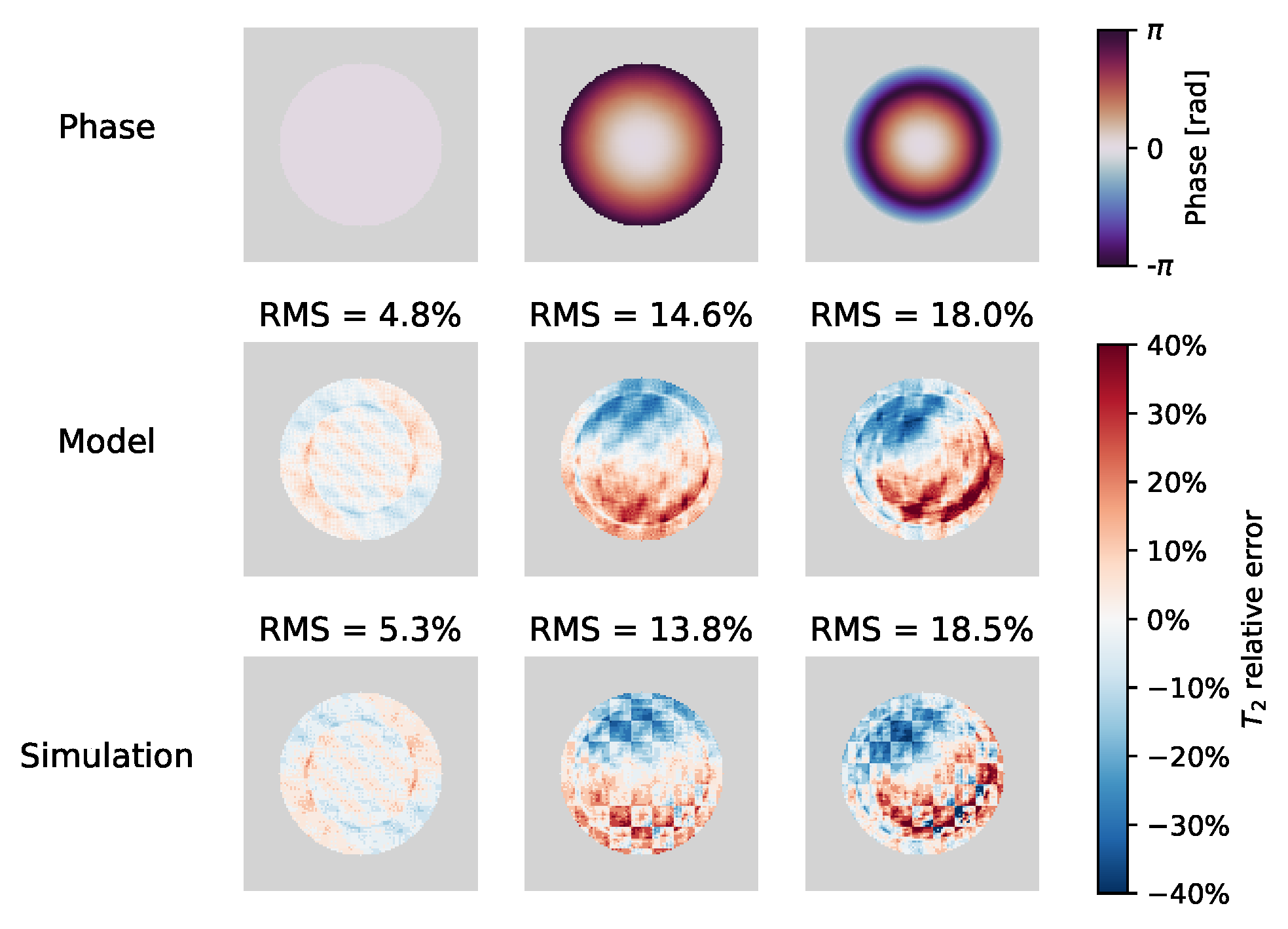
Numerical simulations using a chequerboard-like phantom were performed to validate the implementation of the model by comparing it to a brute force approach (simulated time-frame images, undersampled and reconstructed with zero-filled NUFFT-reconstruction).
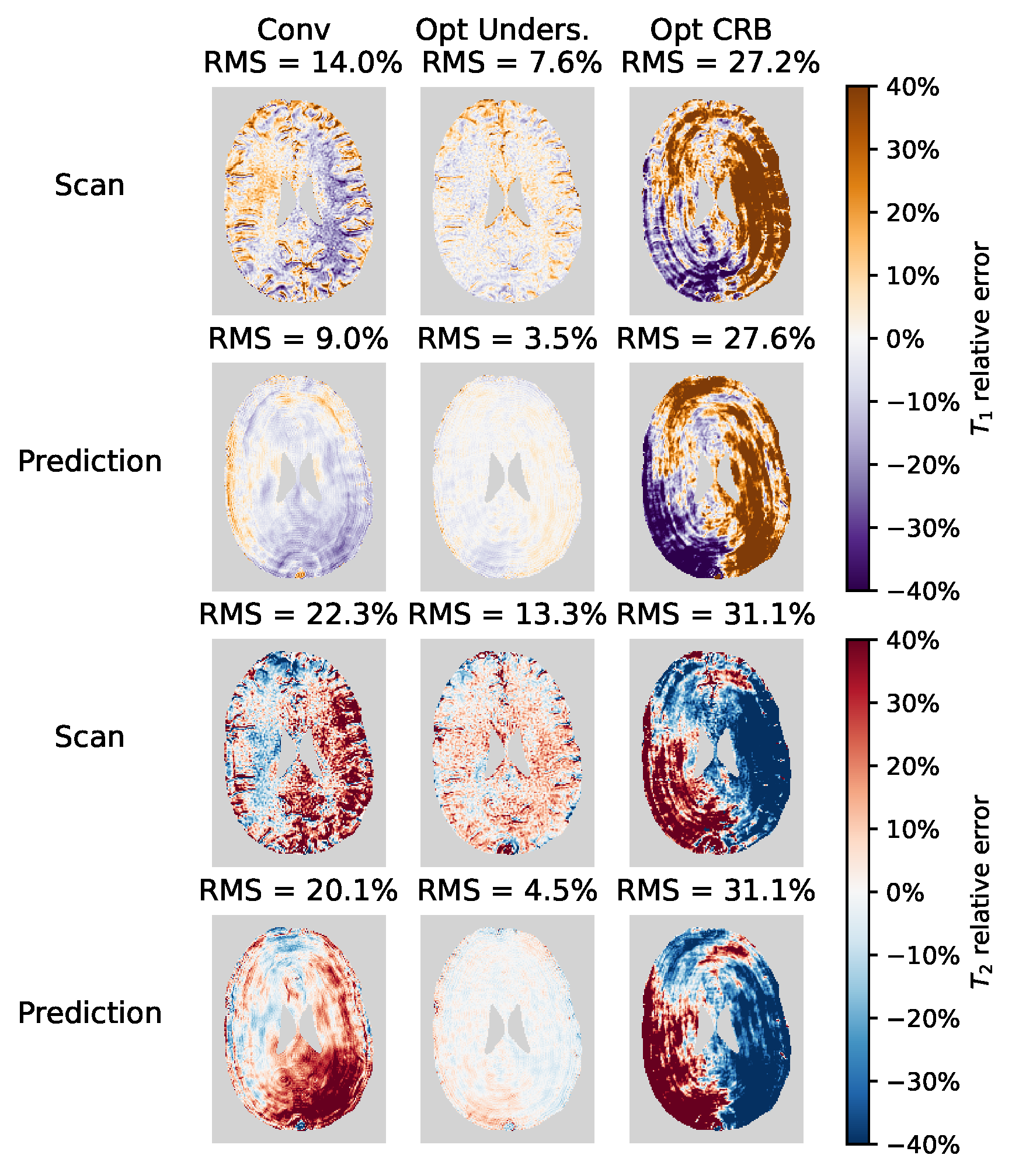
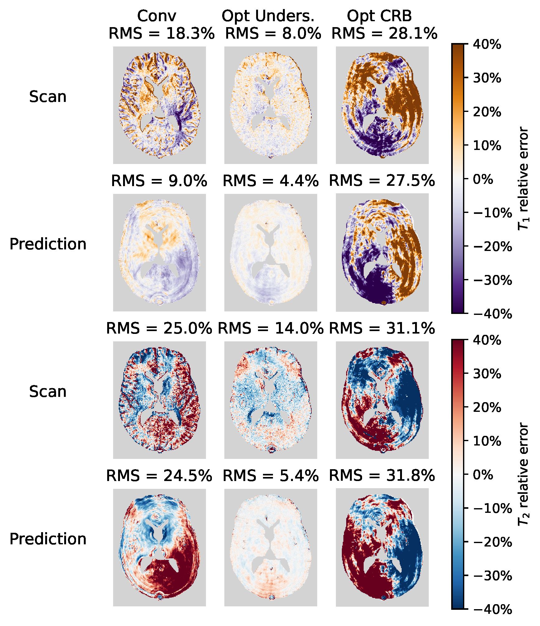
In vivo brain scans were acquired for two healthy volunteers using a 3.0 T Philips Ingenia MRI-scanner (Best, The Netherlands) for further validation and comparison. Two slices were acquired with FOV=$$$224\text{mm}\times224\text{mm}$$$,$$$\,1\text{mm}\times1\text{mm}$$$ in plane resolution, $$$5\text{mm}$$$ slice thickness and $$$20\text{mm}$$$ slice gap. Fully-sampled and undersampled(1/32) acquisitions with incremental $$$\frac{2\pi}{32}$$$-rotation and constant-density spirals were performed.
After dictionary matching, relative errors maps were calculated using the fully-sampled scans as reference.
Results and discussion
In simulations, error maps from the implemented model and brute force approach show a close resemblance(Fig.1). The signal phase has a strong effect on the estimated $$$T_2$$$-errors and leads to unexpected asymmetries, dependent on the spiral shape and orientation.The conventional and optimised sequences together with the evolution of the transverse magnetisation are shown in Fig.2.
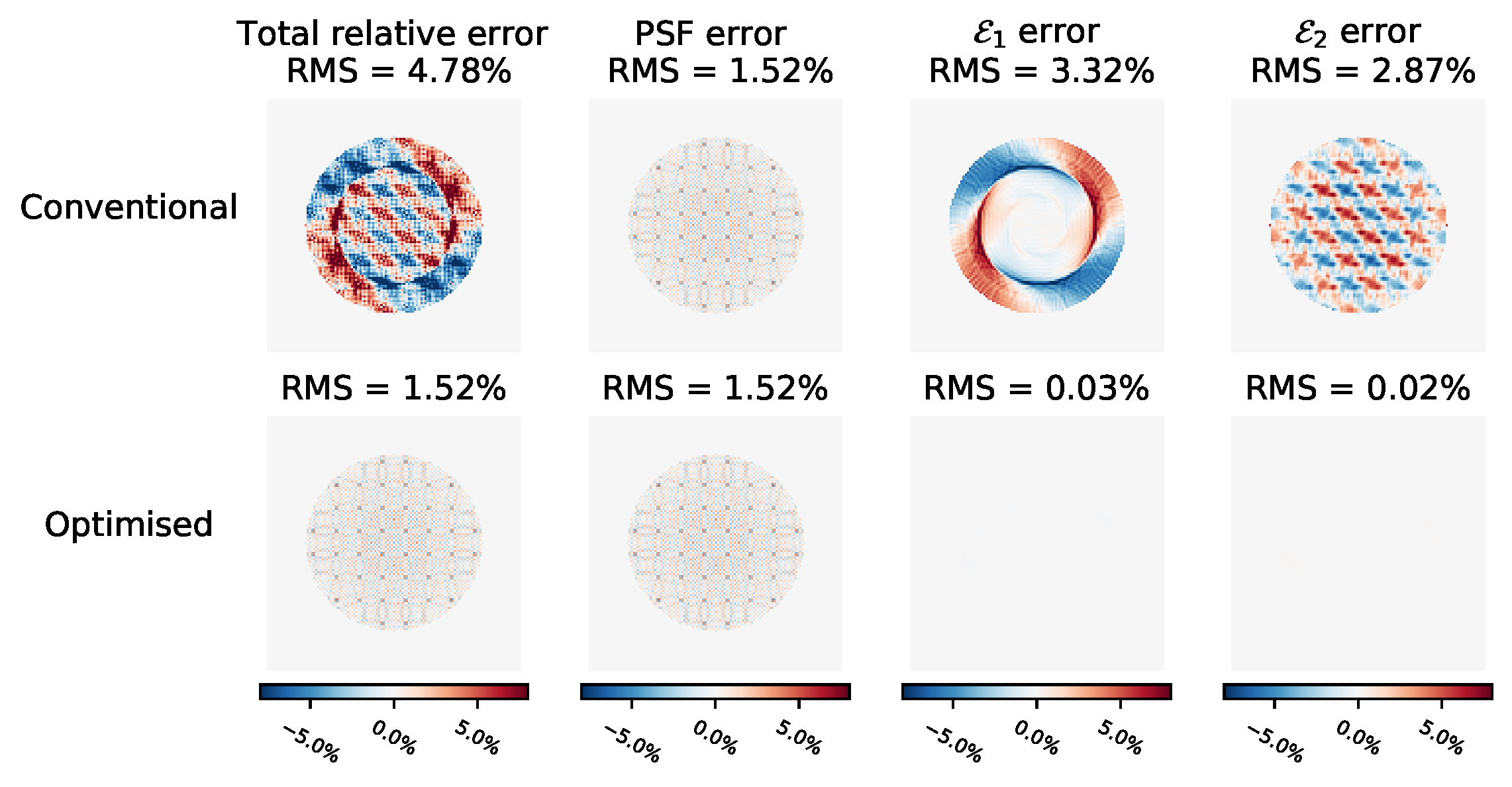
The individual components of the undersampling error are shown in Fig.3(see Theory). The two error terms are almost reduced to zero. Note that the chequerboard pattern is only visible in the $$$\mathcal{E}_2$$$-error as this depends on $$$\boldsymbol{\theta}$$$.
In vivo, a strong reduction in both $$$T_1$$$ and $$$T_2$$$-error can be observed when using the undersampling optimised sequence(Fig.4 and Fig.5). To our surprise, the CRB-optimised sequence performed worse than the conventional sequence. We hypothesise that this is caused by the strong signal variations in the first time points(Fig.2). The error predictions are in good agreement with the measured errors when undersampling is the dominant error term (Conv and Opt CRB).
Recent similar work on MRF-sequence optimisation9 applied a spatial-temporal separation of the problem using a simplified brain phantom with three different tissues as ground-truth to achieve feasible computation times. The here used framework allows for the use of in vivo maps as ground-truth, allowing a more flexible choice of regions of interest. We observed a similar importance of signal phase and the ability to reduce errors influenced by this phase variation as the aforementioned work.
A limitation of this work is the assumption of zero-filled reconstruction. More advanced reconstructions10,11 might reduce undersampling artefacts, making the interplay between undersampling and flip angle patterns less obvious at cost of increased reconstruction times.
Conclusion
The performed MRF-sequence optimisation showed a clear reduction in errors introduced by undersampling compared to a conventional sequence and a Cramér-Rao Bound optimised sequence.Acknowledgements
This research was partly funded by the Medical Delta consortium, a collaboration between the Delft University of Technology, Leiden University, Erasmus University Rotterdam, Leiden University Medical Center and Erasmus Medical Center.
The authors want to thank Emiel Hartsema, Thijs van Osch and Kirsten Koolstra for fruitful discussions and/or help during acquisitions. Furthermore the authors want to acknowledge the contribution by C.C. Stolk and A. Sbrizzi as they introduced the model on which the optimisations are based.
References
- Ma, D.; Gulani, V.; Seiberlich, N.; Liu, K.; Sunshine, J. L.; Duerk, J. L.; Griswold, M. A. Magnetic Resonance Fingerprinting. Nature 2013, 495, 187–192, DOI: 10.1038/nature11971.
- McGivney, D. F.; Boyacıoglu, R.; Jiang, Y.; Poorman, M. E.; Seiberlich, N.; Gulani, V.; Keenan, K. E.; Griswold, M. A.; Ma, D. Magnetic resonance fingerprinting review part 2: Technique and directions. Journal of Magnetic Resonance Imaging 2019, 51, 993–1007, DOI: 10.1002/jmri.26877.
- Zhao, B.; Haldar, J. P.; Liao, C.; Ma, D.; Jiang, Y.; Griswold, M. A.; Setsompop, K.; Wald, L. L. Optimal Experiment Design for Magnetic Resonance Fingerprinting: Cramér-Rao Bound Meets Spin Dynamics. IEEE Transactions on Medical Imaging 2019, 38, 844–861, DOI: 10.1109/TMI.2018.2873704.
- Sommer, K.; Amthor, T.; Doneva, M.; Koken, P.; Meineke, J.; Börnert, P. Towards predicting the encoding capability of MR fingerprinting sequences. Magnetic Resonance Imaging 2017, 41, 7-14, DOI: 10.1016/j.mri.2017.06.015.
- C. C. Stolk; Sbrizzi, A. Understanding the Combined Effect of k-Space Undersampling and Transient States Excitation in MR Fingerprinting Reconstructions. IEEE Transactions on Medical Imaging 2019, 38, 2445–2455, DOI: 10.1109/TMI.2019.2900585.
- Jiang, Y.; Ma, D.; Seiberlich, N.; Gulani, V.; Griswold, M. A. MR fingerprinting using fast imaging with steady state precession (FISP) with spiral readout. Magnetic Resonance in Medicine 2015, 74, 1621–1631, DOI: 10.1002/mrm.25559.
- Hennig, J. Echoes—how to generate, recognize, use or avoid them in MR-imaging sequences. Part I: Fundamental and not so fundamental properties of spin echoes. Concepts in Magnetic Resonance 1991, 3, 125–143, DOI: 10.1002/cmr.1820030302.
- Weigel, M. Extended phase graphs: Dephasing, RF pulses, and echoes - pure and simple. Journal of Magnetic Resonance Imaging 2015, 41, 266–295, DOI: 10.1002/jmri.24619.
- Jordan, S. P.; Hu, S.; Rozada, I.; McGivney, D. F.; Boyacioglu, R.; Jacob, D. C.; Huang, S.; Beverland, M.; Katzgraber, H. G.; Troyer, M.; Griswold, M. A.; Ma, D. Automated design of pulse sequences for magnetic resonance fingerprinting using physics-inspired optimization. Proceedings of the National Academy of Sciences 2021, 118, DOI: 10.1073/ pnas.2020516118.
- Assländer, J.; Cloos, M. A.; Knoll, F.; Sodickson, D. K.; Hennig, J.; Lattanzi, R. Low Rank Alternating Direction Method of Multipliers Reconstruction for MR Fingerprinting. Magnetic resonance in medicine 2018, 79, 83–96, DOI: 10.1002/mrm.26639.
- Cruz, G. L. d.; Bustin, A.; Jaubert, O.; Schneider, T.; Botnar, R. M.; Prieto, C. Sparsity and locally low rank regularization for MR fingerprinting. Magnetic Resonance in Medicine 2019, 81, 3530–3543, DOI: https://doi.org/10.1002/mrm.27665.
Figures