Introduction

Non-Cartesian trajectories provide rapid imaging¹ and robustness to patient motion², but can be susceptible to off-resonance blurring, especially when readout durations are long. Several analytical methods have been developed for off-resonance correction, but are mostly computationally slow and require accurate field map estimates, often via additional scans. Recent works have considered deep-learning solutions^3-5 which use convolutional neural networks (CNN) to deblur images directly or estimate field maps. However, these methods use real MRI data for training and do not leverage the physics behind off-resonance blurring.

We propose a physics-inspired unrolled-deep-learning framework for off-resonance correction. Our model enforces data consistency with a forward model that includes coil sensitivities, multi-frequency bins, and non-uniform Fourier transforms. The model is trained end-to-end using only synthetic random field maps, coil sensitivities, and noise-like images, with the aim of learning to reverse off-resonance irrespective of the type of imaging and hence generalize to any anatomy and contrast without retraining.

Methods

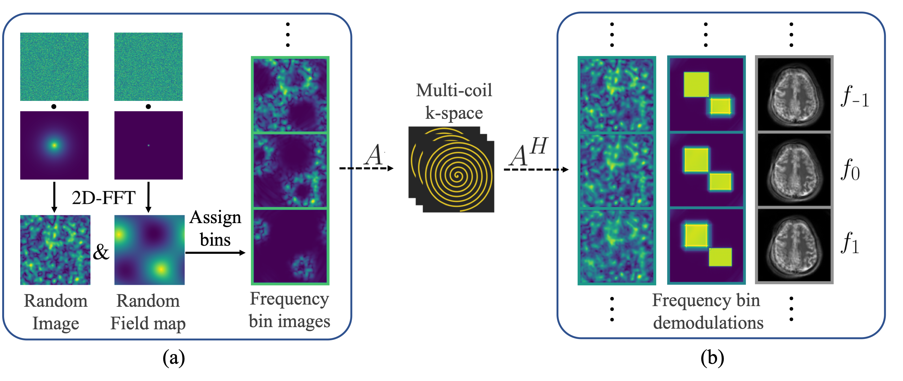
Forward Model definition

We aim to solve for $$$x$$$ such that $$$A(x)=y$$$, where $$$A$$$ is the forward model, $$$y$$$ the multi-coil k-space measurements, and $$$x$$$ the clean image for each frequency bin. We approximate the forward model as follows (Figure 1): $$A=\Sigma\cdot M\cdot F\cdot S$$ where $$$M=\exp{(j\cdot2\pi\cdot f\cdot t)}$$$.

We model the image as a stack of sharp images at different resonant frequencies around the center Larmor frequency, each containing the region of the object that is resonant. The coil images for each frequency bin are obtained by multiplication with coil sensitivity maps ($$$S$$$). Finally, a density compensated NUFFT ($$$F$$$) calculates the non-Cartesian k-space for each bin, which is then modulated at the corresponding frequency ($$$M$$$). These differently modulated k-spaces are then summed ($$$\Sigma$$$) to obtain a complete representation of the acquired multi-coil k-space.

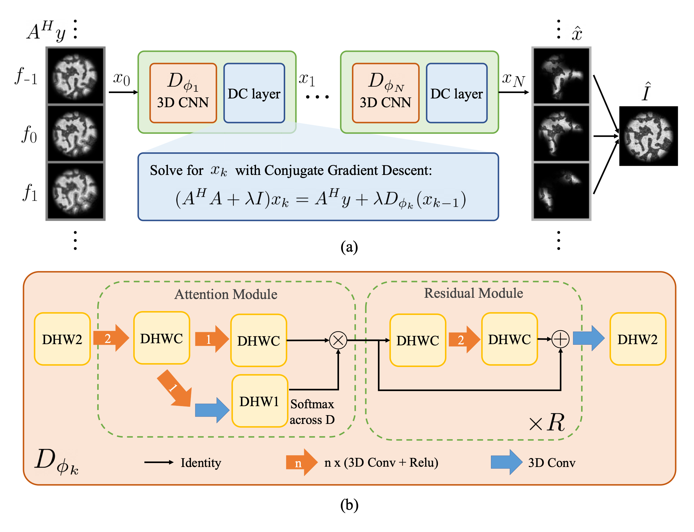
This problem is ill-posed, and hence, we incorporate a neural network for regularization. We take a MoDL-inspired⁶ approach, an unrolled iterative model that is trained end-to-end (Figure 3a). The input to our model is a stack of images demodulated at multiple frequencies obtained from the adjoint operator $$$A^H$$$ on raw multi-coil kspace. Regions of the object are sharp at the frequency bin corresponding to its local resonant frequency, while other off-resonant regions blur on top (Figure 2b). The objective of our model is to obtain a clear image at each frequency bin, as well as a final combined image without off-resonance blurring.

CNN architecture

The 3D CNN architecture is depicted in Figure 3b. The network takes the complex images obtained from applying $$$A^H$$$ to multi-coil k-space, with the real and imaginary parts as different channels. Convolutions are across image dimensions and frequency bins. We use a combination of an attention module across frequencies and residual modules⁷. The attention module allows the network to focus on features from a certain frequency range at each spatial location. After the attention module, $$$R$$$ residual blocks follow, and a final convolution outputs the cleaner complex images at each frequency.

Training data simulation

Inspired by [8], all the training data corresponds to simulated synthetic random field maps, coil sensitivities, and noise-like images with statistics (smoothness) mimicking natural signals. Random images and field maps are generated by applying a 2D-FFT to exponentially weighted random complex data, where the weighting radius determines the level of smoothness. Similarly, random sensitivity maps are generated from weighted random SPIRiT kernels⁹. The images at multiple bins are obtained by blurring a random image $$$I$$$ into the bins according to a random field map $$$F$$$ and bin frequency values, obtaining $$$x$$$. Our sensitivity maps and $$$x$$$ are fed to the forward model to obtain our multi-coil k-space $$$y$$$.

From here, we have all the elements to supervise our model. The model’s output $$$\hat{x}$$$ can be supervised with the ground truth $$$x$$$, as well as the combined output image $$$\hat{I}=\sum_i\hat{x}_{f_i}$$$ can be supervised with $$$I$$$. Additionally, we can aid learning by supervising the attention maps with the frequency bin weights obtained from the field map.

Experiments & Results

To evaluate our approach, we trained a model simulating a spiral trajectory with 4 interleaves, 10.72ms readout, $$$2.2\text{mm}^2$$$ resolution, and off-resonance field map in the range of -200Hz/200Hz (corresponding to 2.15 phase cycles). We picked 11 frequency bins in the -200Hz/200Hz range (step of 40Hz between bins) for our model approximation, and simulated 6 coils during training. We used Adam¹⁰ optimizer with L1 losses. For our unrolled model, we used 4 unrolls, 2 residual blocks on each network, and 12 conjugate gradient iterations with $$$\lambda=1$$$.

Results on noise data and real brain images with simulated synthetic off-resonance are shown in Figure 4. Results from evaluating our noise-trained network on acquired phantom and in-vivo brain data are shown in Figure 5. We used a spiral GRE sequence with a spectral-spatial pulse for water-only excitation. We scanned with the same readout trajectory as in training, as well as with a higher-resolution ($$$1\text{mm}^2$$$) scan with a different spiral trajectory (13 interleaves, 10.72ms readout). Sensitivity maps for the acquired data were estimated with ESPIRiT¹¹ using BART¹².

Conclusion

We introduce a physics-inspired, unrolled-deep-learning framework for off-resonance correction. Our model is trained purely on synthetic multi-coil data in order to generalize to any anatomy and contrast without retraining.

Acknowledgements

No acknowledgement found.